#Cloud Optimized GeoTIFF

2 posts

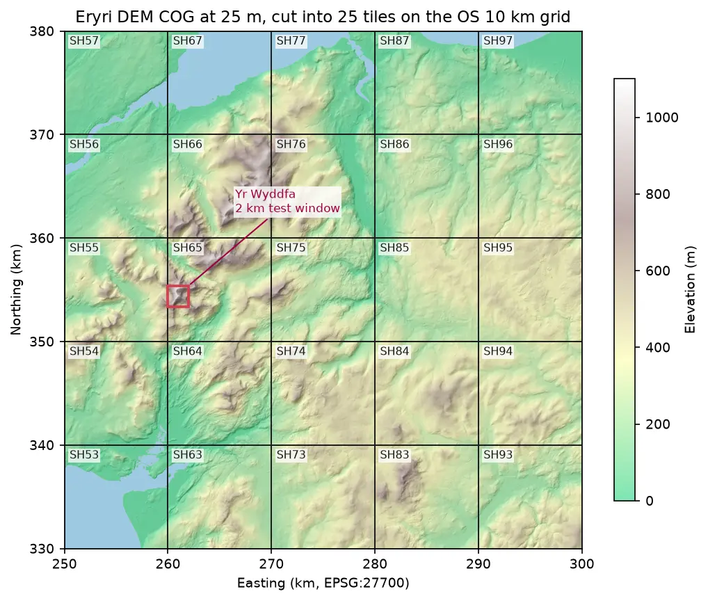
Hillshaded elevation map of Eryri at 25 m in British National Grid, coloured from green lowland to white summits, divided into 25 labelled 10 km squares from SH53 to SH97, with a red 2 km box marking the Yr Wyddfa test window

Tutorial Python Part 1 of 2

Cloud Optimised GeoTIFFs in Python: reproject, mosaic and validate a COG

Mosaic four Copernicus DEM GLO-30 tiles straight from AWS with rasterio, reproject them to British National Grid, write a validated Cloud Optimised GeoTIFF with rio-cogeo, and measure exactly how many bytes HTTP range requests fetch.
Intermediate 12 min read

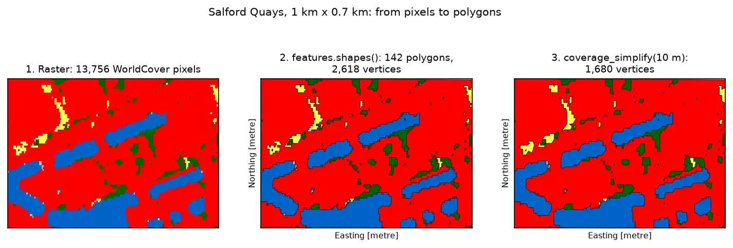
Three panels of the same 1 km by 0.7 km area at Salford Quays. Left: square WorldCover pixels, mostly red built-up land with blue dock basins and small green and yellow patches. Middle: the same area as 142 polygons with black outlines that follow the pixel staircase. Right: the polygons after coverage simplification at 10 m, with smoother outlines and no gaps between them.

Tutorial Python Part 3 of 3

Raster to vector in Python: polygonize with rasterio, rasterize boundaries and convert a GeoTIFF to a Cloud Optimized GeoTIFF

Convert raster to vector in Python with rasterio.features.shapes on 10 m ESA WorldCover for Greater Manchester: polygonize water and built-up land, fix invalid polygons, simplify without gaps, rasterize ONS district boundaries for land-cover shares, then write and validate a Cloud Optimized GeoTIFF with rio-cogeo and measure HTTP range reads.

Intermediate 14 min read