Python

GeoPandas, rasterio, xarray, STAC and OSMnx workflows you can run end-to-end.

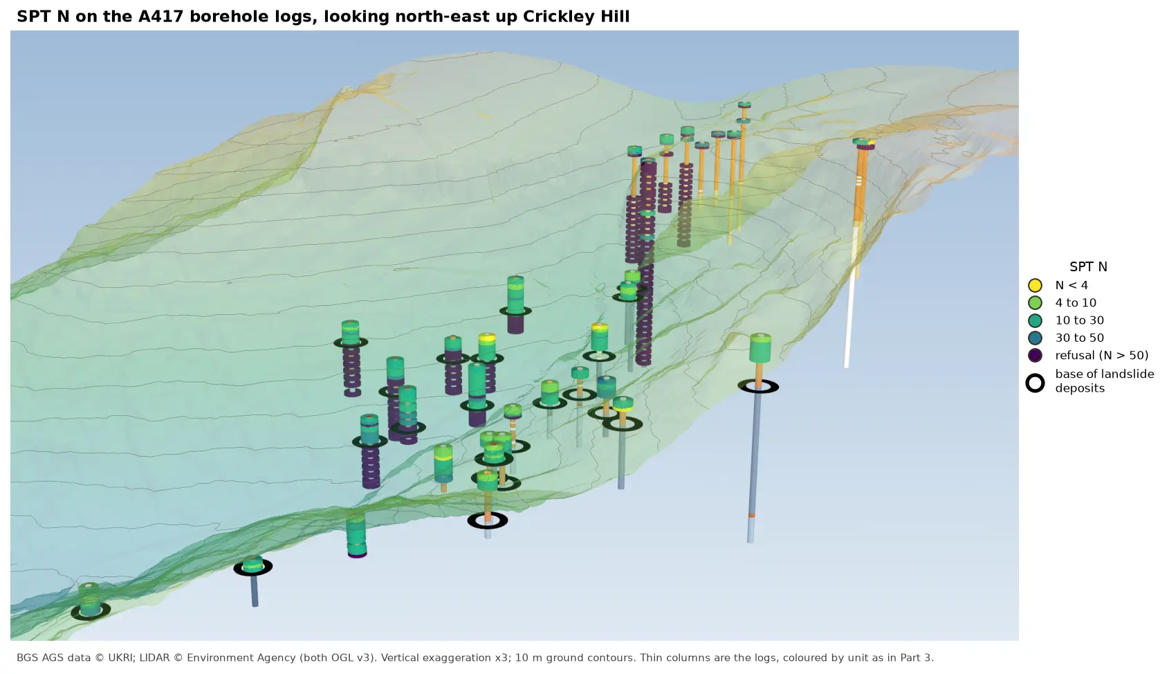
3D view looking north-east up Crickley Hill over semi-transparent LIDAR terrain with 10 m contours. Thin borehole logs coloured by unit carry stacks of coloured discs, one per SPT: yellow and green discs for low N-values near the top of the holes on the escarpment, changing to dark purple refusal discs below black rings that mark the base of the landslide deposits. On the plateau at the top right, the holes turn purple within a few metres of the surface.

Tutorial Python Part 6 of 7

Visualising SPT N-values from AGS4 data in Python

Read the Standard Penetration Tests (ISPT) from a real AGS4 file, separate full tests from refusals, find the stratum each test was made in, and show the N-values four ways: by unit against elevation, across the base of a landslide, as coloured discs on 3D borehole logs over LIDAR terrain, and as a map of the depth to the first refusal.
Intermediate 10 min read

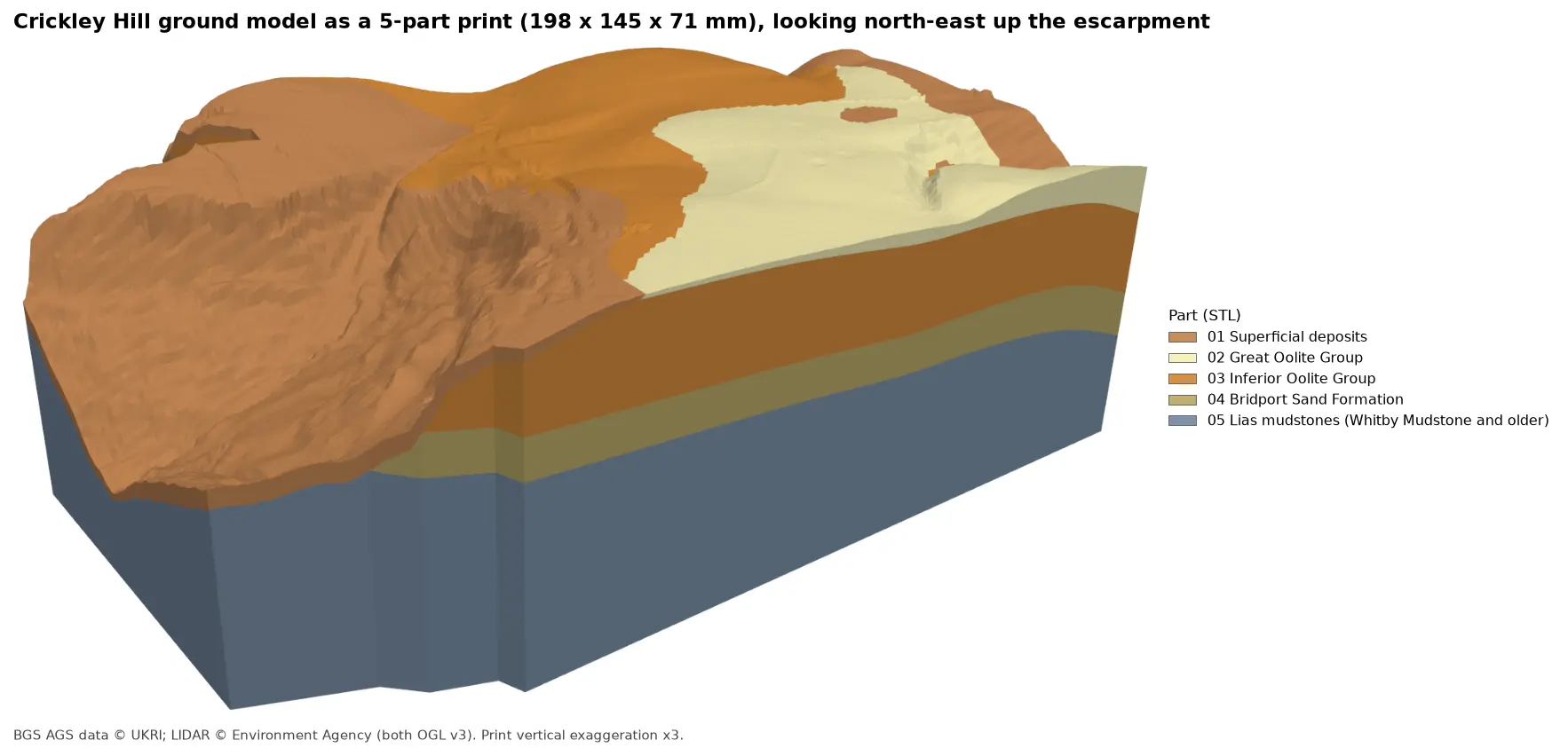
Rendered 3D print of the Crickley Hill ground model, 198 by 145 by 71 mm, looking north-east up the escarpment. Brown superficial deposits cover the western slope, orange Inferior Oolite forms the scarp and plateau, pale yellow Great Oolite caps the south-east, and the side walls show a band of olive Bridport Sand over blue-grey Lias mudstones.

Tutorial Python Part 7 of 7

3D-print a geological ground model: one watertight STL per stratum

Turn the kriged stratum surfaces from Part 5 into a multi-material 3D print of the Cotswold escarpment at Crickley Hill. Cut a window, decide what is too thin to print, build one solid per unit with mesh booleans, prove the parts fit exactly and are watertight, and write five STLs and a colour 3MF for AMS and MMU printers.

Advanced 11 min read

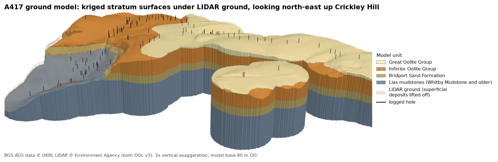
3D block model of the A417 ground model looking north-east up Crickley Hill: blue-grey Lias mudstones form the vale and the lower walls, under a band of olive Bridport Sand, a thick orange band of Inferior Oolite and pale yellow Great Oolite on the plateau. Black vertical lines mark the logged boreholes, and a faint buff skin shows the LIDAR ground lifted off the superficial deposits.

Tutorial Python Part 5 of 7

A 3D ground model from AGS4 boreholes: kriged stratum surfaces in Python

Pick rockhead and the top and base of the key formations from real AGS4 logs, krige them into stratum surfaces under Environment Agency LIDAR ground, and build a 3D ground model of the A417 escarpment in PyVista. Then test it: leave-one-out cross-validation at every borehole, kriging standard deviation maps, a check against every hole that stops short of a surface, and proof that no surface crosses another.

Advanced 15 min read

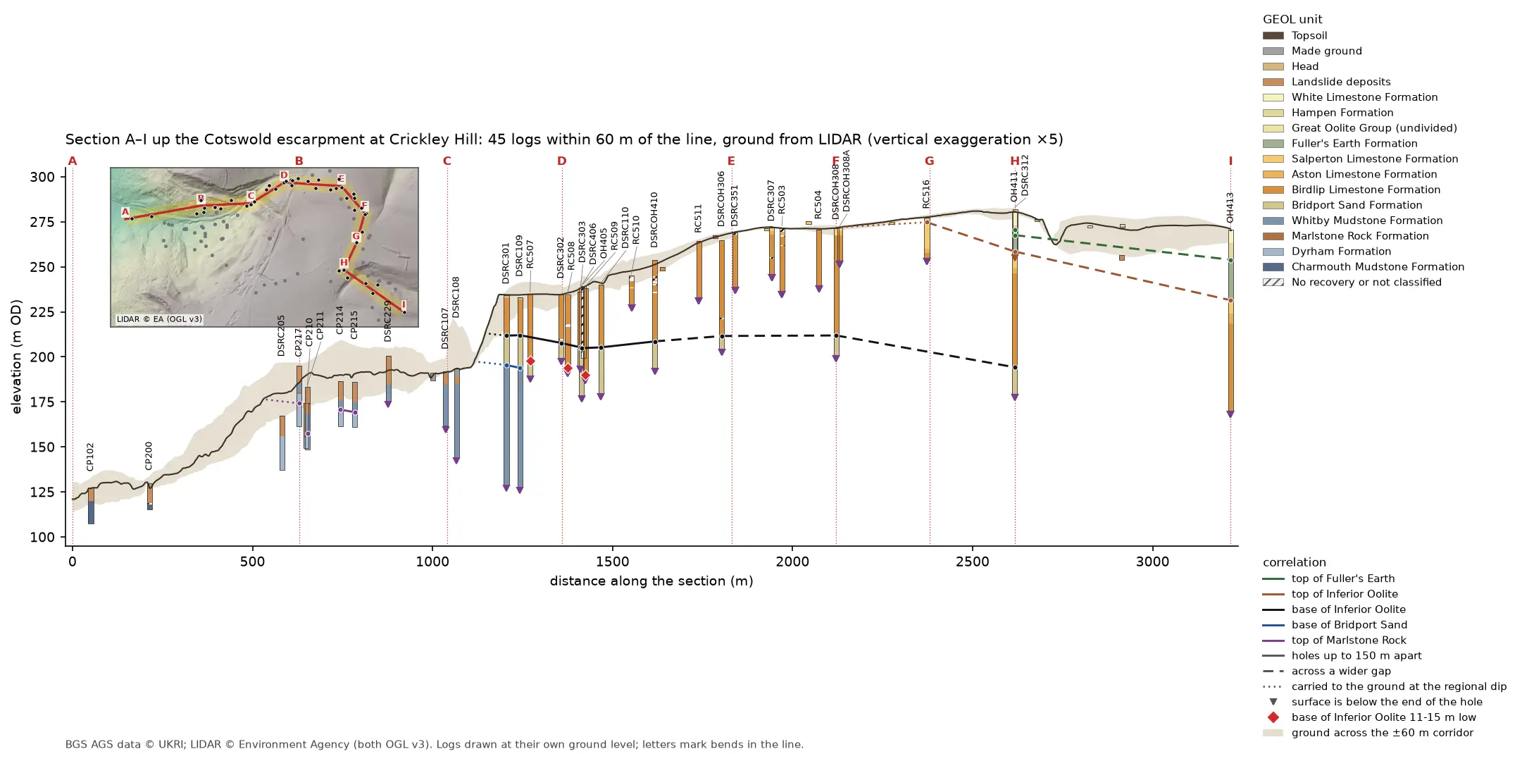
Geological cross-section 3.2 km long from the vale at A, up the Cotswold escarpment at Crickley Hill, to the plateau at I. A dark LIDAR ground line climbs from 121 to 281 m OD over a buff band showing the ground across the corridor. Forty-five strip logs hang below it, coloured by formation: blue-grey Lias mudstone in the vale, orange Inferior Oolite limestone on the escarpment and green Fuller's Earth on the plateau. Coloured lines join the contacts between holes, and red diamonds mark three holes where the base of the limestone is 11 to 15 m low. A map inset at top left shows the bent section line and its corridor on a LIDAR hillshade.

Tutorial Python Part 4 of 7

A geological cross-section from AGS4 boreholes and LIDAR in Python and QGIS

Draw a 3.2 km geological cross-section up the Cotswold escarpment from real AGS4 borehole logs, with the ground profile from Environment Agency LIDAR. Project every hole in a corridor onto the line, pick and correlate the contacts, and measure how much of each correlation line rests on a log and how much is inferred. Then draw the same section with the QGIS elevation profile.

Intermediate 15 min read

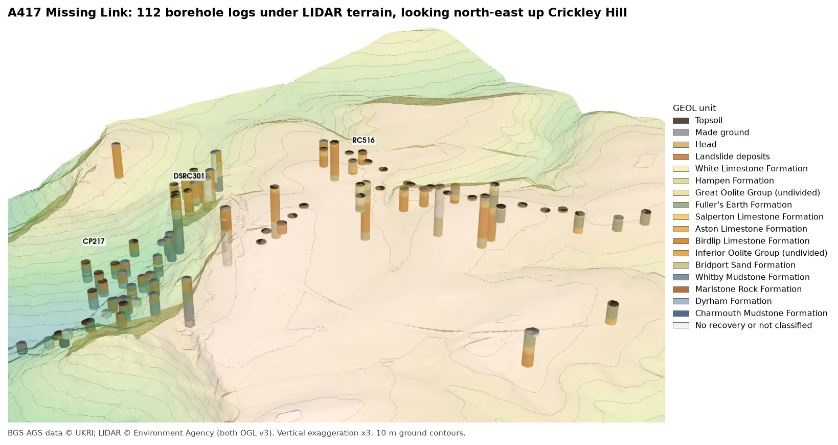
3D view looking north-east up Crickley Hill: LIDAR terrain shaded from green in the vale to buff on the plateau, with 10 m contours, and 112 borehole logs drawn as vertical cylinders coloured by formation. Blue-grey Lias mudstones fill the holes in the vale, orange Inferior Oolite limestones those on the escarpment, and green Fuller's Earth those on the plateau.

Tutorial Python Part 3 of 7

3D borehole logs from AGS4 data in PyVista and QGIS

Build every borehole log in a real AGS4 file as coloured 3D cylinders at their true elevation under Environment Agency LIDAR terrain with PyVista, then style the same intervals in the QGIS 3D map view. Along the way, test whether neighbouring logs agree, and find a block of ground at the top of Crickley Hill where they don't.

Intermediate 12 min read

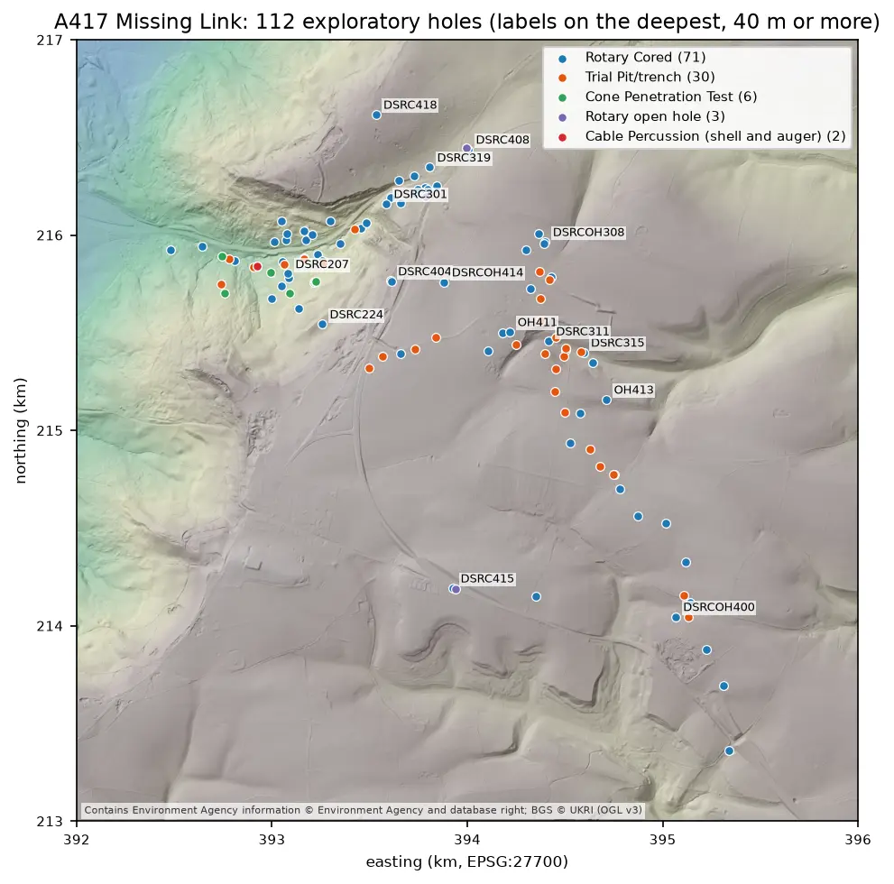
Map of the A417 Missing Link ground investigation on a grey LIDAR hillshade: 112 coloured points for rotary cored boreholes, trial pits, cone penetration tests, open holes and cable percussion boreholes, strung along the road corridor from the vale in the north-west, up the escarpment and south-east across the plateau, with the deepest holes labelled.

Tutorial Python Part 2 of 7

Boreholes on a map: AGS4 locations in British National Grid with QGIS

Turn the LOCA group of a real AGS4 file into points in British National Grid, see what happens when the CRS is wrong, summarise each hole's geology from GEOL, check every ground level against Environment Agency LIDAR, and build a QGIS project with labels and a map tip that shows the borehole log.

Intermediate 8 min read

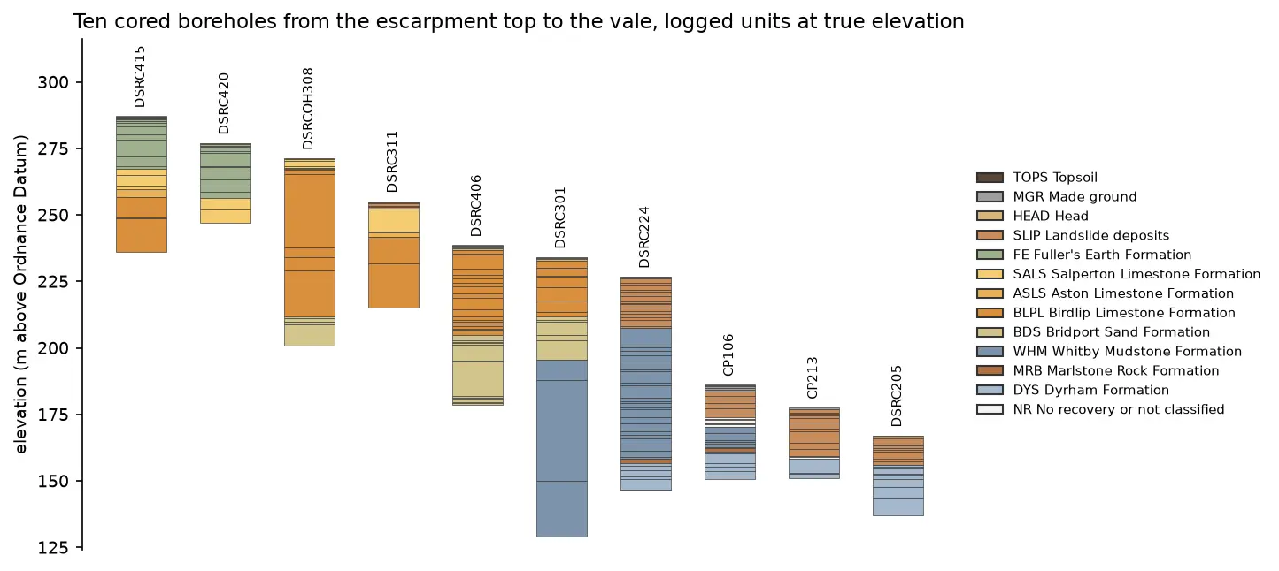
Ten borehole strip logs plotted at true elevation, stepping down from about 287 m above Ordnance Datum on the left to about 167 m on the right. Fuller's Earth and limestone units at the top give way to Bridport Sand, then thick blue-grey Whitby Mudstone and Dyrham Formation in the lower holes.

Tutorial Python Part 1 of 7

Read and validate AGS4 ground investigation data with Python

Find a real ground investigation in the British Geological Survey's AGS archive, download it as AGS4, learn how the file is put together, read it into pandas with python-ags4, fix every error the AGS checker reports, and check that the borehole logs make geological sense. The example is the A417 Missing Link at Crickley Hill.

Intermediate 12 min read

Tutorial Python Part 5 of 5

Tiling a large 3D-printed terrain model: jigsaw joints and dowel pins in Python

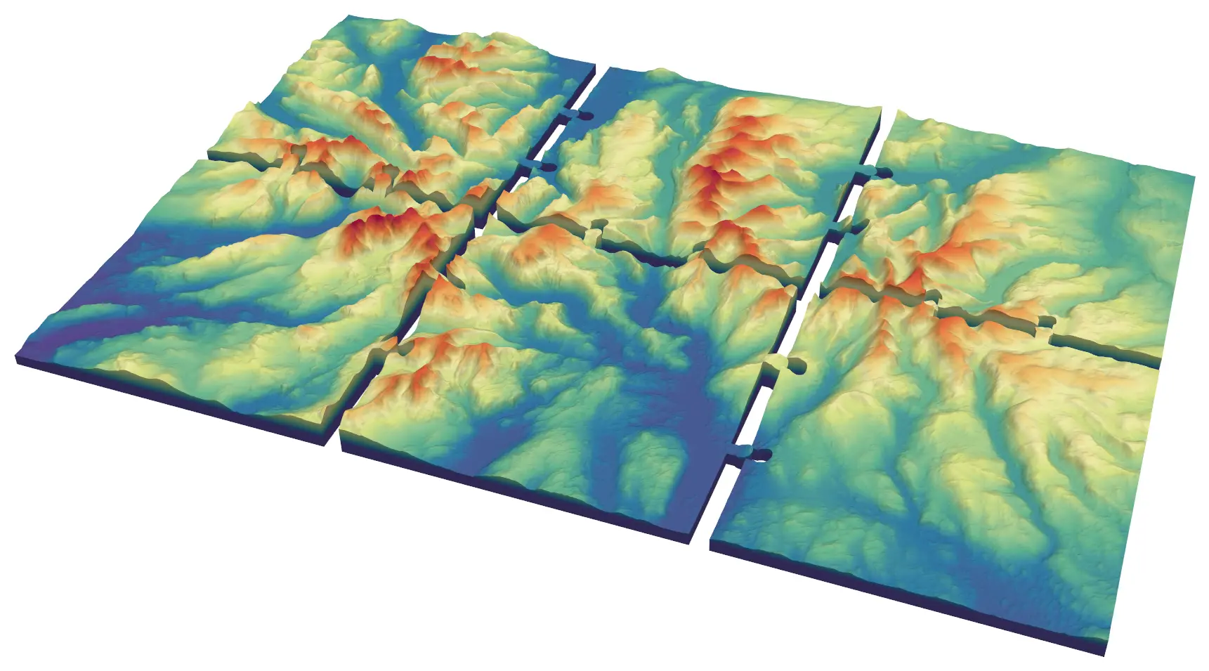
Split a 45 × 30 km model of the central Lake District into six interlocking 150 mm tiles from Copernicus GLO-30, with jigsaw knobs and a 0.2 mm printing clearance or straight edges and filament dowels, and prove every tile is watertight and fits its neighbours.

Advanced 9 min read

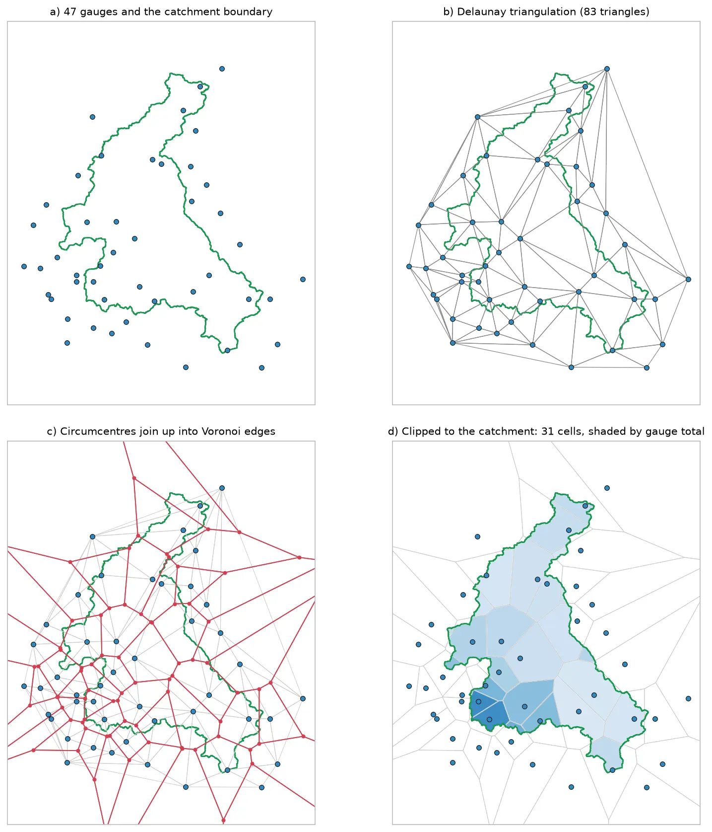
Four panels showing how Voronoi polygons are built for 47 rain gauges around the River Eden catchment: the gauges and the catchment outline, their Delaunay triangulation, the triangle circumcentres joined into red Voronoi edges, and the cells clipped to the catchment and shaded by each gauge's rainfall.

Tutorial Python

Voronoi (Thiessen) polygons in Python: catchment rainfall from EA rain gauges and fire station areas in Cumbria

Build Voronoi (Thiessen) polygons in Python with shapely and GeoPandas, clipped to a real boundary. Compute Thiessen-weighted catchment rainfall for the River Eden from Environment Agency rain gauge readings, check the gauges, compare with the gauge average and IDW, then compare Voronoi 'nearest fire station' areas in Cumbria with drive-time service areas from OpenStreetMap.

Intermediate 15 min read

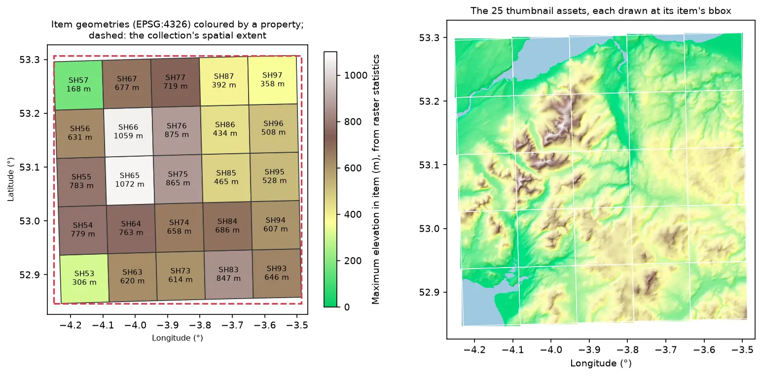
Two maps of Eryri in longitude and latitude. Left: 25 slightly rotated STAC item footprints labelled SH53 to SH97 and coloured by maximum elevation, inside a dashed red collection extent. Right: the 25 hillshaded thumbnail assets drawn at their item bounding boxes, forming one relief map

Tutorial Python Part 2 of 2

Build a STAC catalogue in Python with pystac, rio-stac and pystac-client

Turn 25 Cloud Optimised GeoTIFFs of Eryri into a static STAC catalogue with pystac and rio-stac, validate it against the JSON schemas, query it, serve it as static files, and compare it with the Earth Search and Planetary Computer STAC APIs through pystac-client.

Intermediate 12 min read

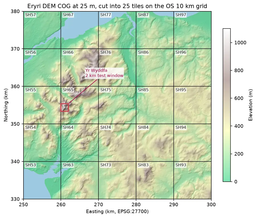
Hillshaded elevation map of Eryri at 25 m in British National Grid, coloured from green lowland to white summits, divided into 25 labelled 10 km squares from SH53 to SH97, with a red 2 km box marking the Yr Wyddfa test window

Tutorial Python Part 1 of 2

Cloud Optimised GeoTIFFs in Python: reproject, mosaic and validate a COG

Mosaic four Copernicus DEM GLO-30 tiles straight from AWS with rasterio, reproject them to British National Grid, write a validated Cloud Optimised GeoTIFF with rio-cogeo, and measure exactly how many bytes HTTP range requests fetch.

Intermediate 12 min read

Tutorial Python

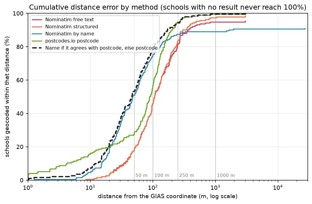
Geocoding in Python: batch and reverse geocoding with geopy, Nominatim and postcodes.io

Batch geocode all 192 open schools in Sheffield in Python with geopy and OpenStreetMap Nominatim (1 request per second, a custom user agent and an on-disk cache) and with postcodes.io bulk postcode lookups, reverse geocode a sample, and measure every method honestly against the Department for Education's own coordinates. Covers free text against structured queries, failure modes, cross-checking two geocoders, and the licensing of geocoded results.

Beginner 14 min read

Tutorial Python

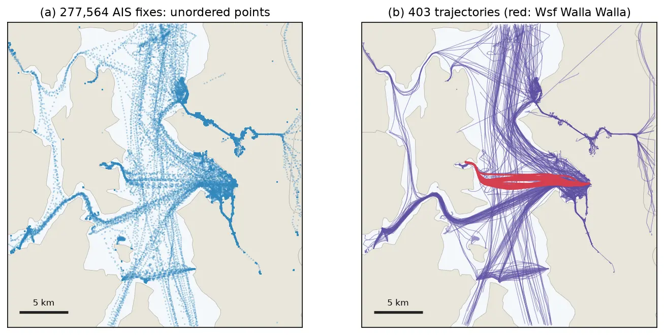
GPS data analysis in Python with MovingPandas: trajectories, speed, stops, generalisation and flow maps

A MovingPandas tutorial on one day of real AIS vessel tracks in Puget Sound: 277,574 GPS fixes from 703 vessels turned into trajectories, with speed and direction, outlier cleaning, stop detection at ferry terminals, splitting into 148 trips, Douglas-Peucker against time-aware generalisation, a flow map of 319 aggregated flows, and reading and writing GPX.

Intermediate 14 min read

Tutorial Python

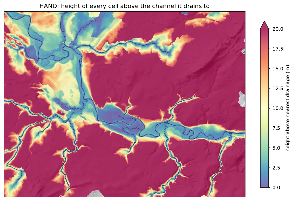
Height above nearest drainage (HAND) flood mapping in Python: the River Severn

Compute height above nearest drainage (HAND) from the Environment Agency LIDAR DTM at 5 m with pysheds, turn it into inundation extents for a range of stage heights on the River Severn between Shrewsbury and Buildwas, relate them to the Buildwas gauge, and score them honestly against the Environment Agency Flood Map for Planning with the hit rate, false-alarm ratio and critical success index.

Intermediate 13 min read

Tutorial Python

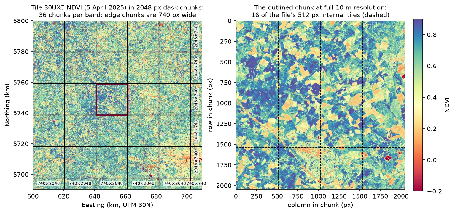
Parallel raster processing in Python with dask and rioxarray: a whole Sentinel-2 tile without running out of memory

Process large satellite rasters in Python with dask and rioxarray. Open eight full Sentinel-2 scenes lazily, choose a chunk size, inspect the task graph, watch CPU and memory with dask diagnostics, compare peak memory with eager NumPy, time chunk sizes and thread counts, and write a median NDVI GeoTIFF to disk chunk by chunk.

Intermediate 17 min read

Tutorial Python

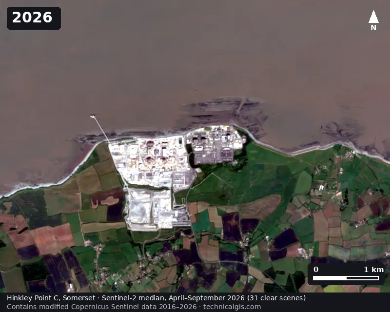
Satellite timelapse in Python: a Sentinel-2 GIF, WebP and MP4 of Hinkley Point C

Create a satellite timelapse in Python from free Sentinel-2 imagery. Select clear scenes with STAC, mask cloud, build one median composite per summer, apply a consistent stretch, add date labels and a scale bar, and export an animated GIF, WebP and MP4 of eleven years of construction at Hinkley Point C.

Intermediate 13 min read

Tutorial Python

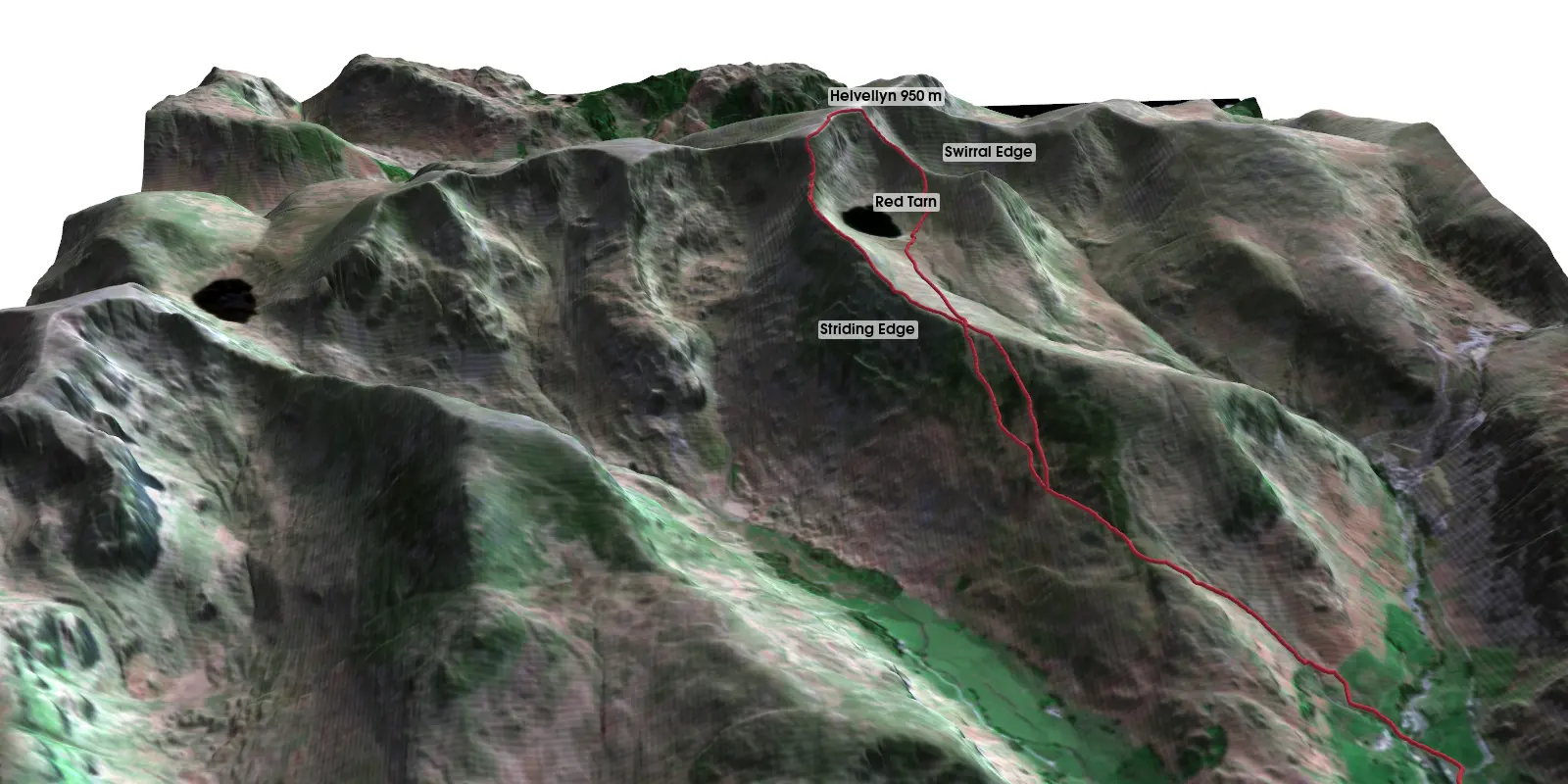
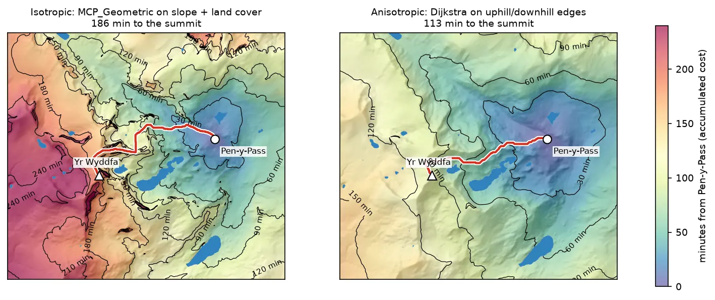
Least-cost path analysis in Python: cost surfaces and walking routes up Yr Wyddfa

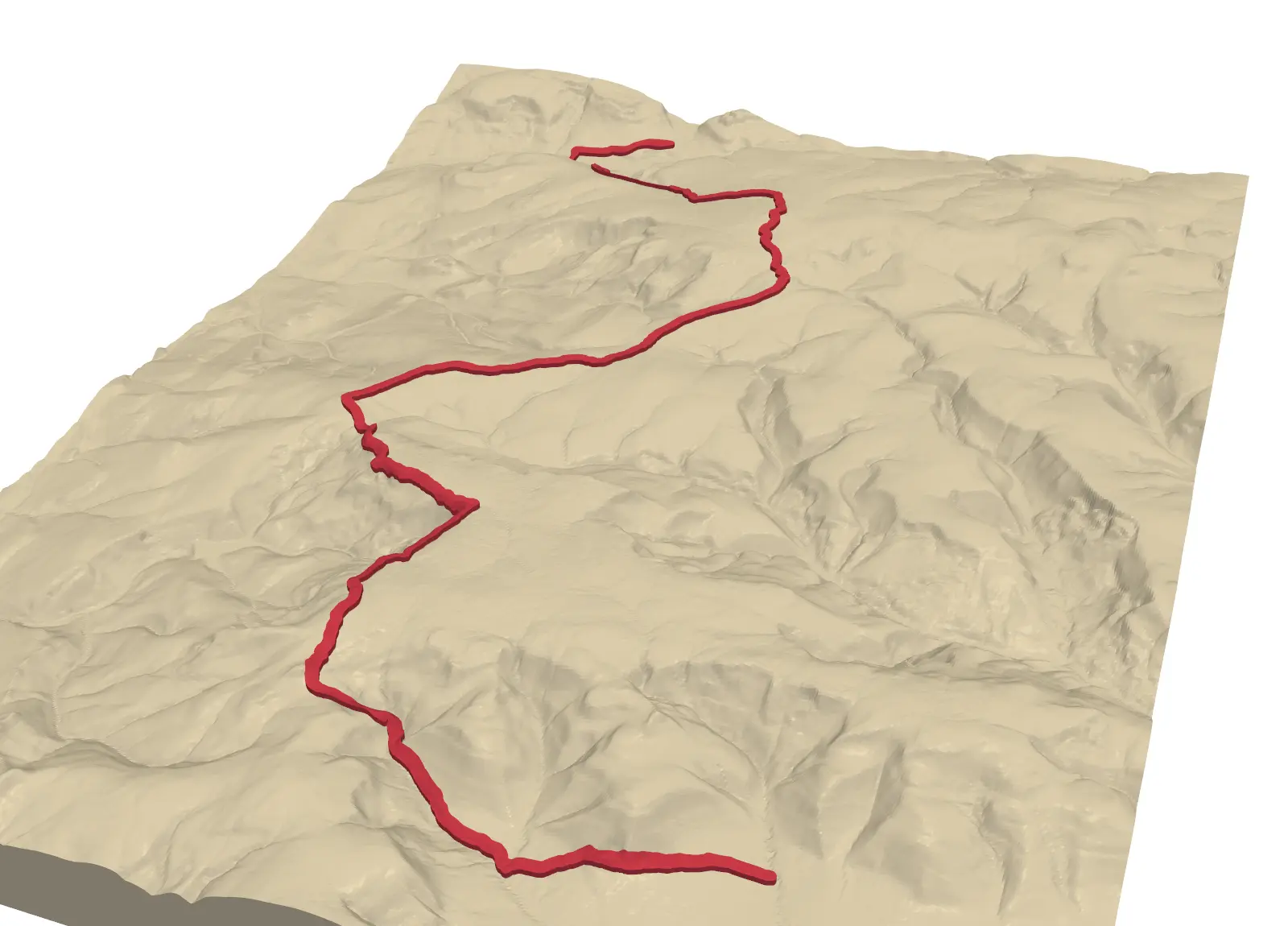
Build a walking cost surface from real slope (Copernicus GLO-30) and land cover (ESA WorldCover), compute the accumulated cost surface and the least-cost path with scikit-image's MCP_Geometric, add a direction-aware Dijkstra version with SciPy, and compare the routes with the straight line and the OpenStreetMap footpaths from Pen-y-Pass to the summit of Yr Wyddfa (Snowdon).

Intermediate 14 min read

Tutorial Python

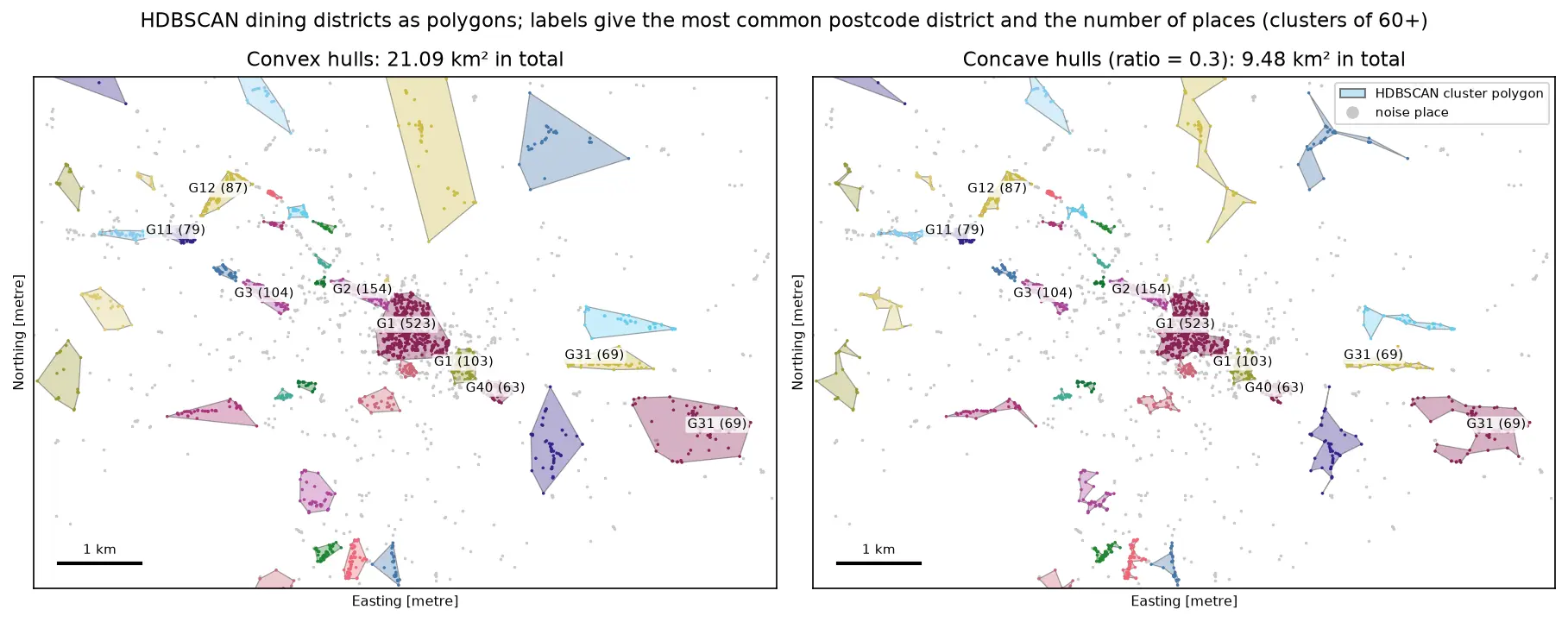
DBSCAN and HDBSCAN spatial clustering in Python: finding Glasgow's dining districts

Cluster GPS and point-of-interest data in Python with DBSCAN and HDBSCAN: use the haversine metric on latitude and longitude or plain metres on a projected grid, choose eps with a k-distance plot, handle variable density with HDBSCAN, draw convex and concave hull polygons, treat noise properly, read silhouette and DBCV with care, and scale up with a BallTree. Uses 3,950 real Overture Maps restaurants, cafés and bars in Glasgow.

Intermediate 18 min read

Tutorial Python

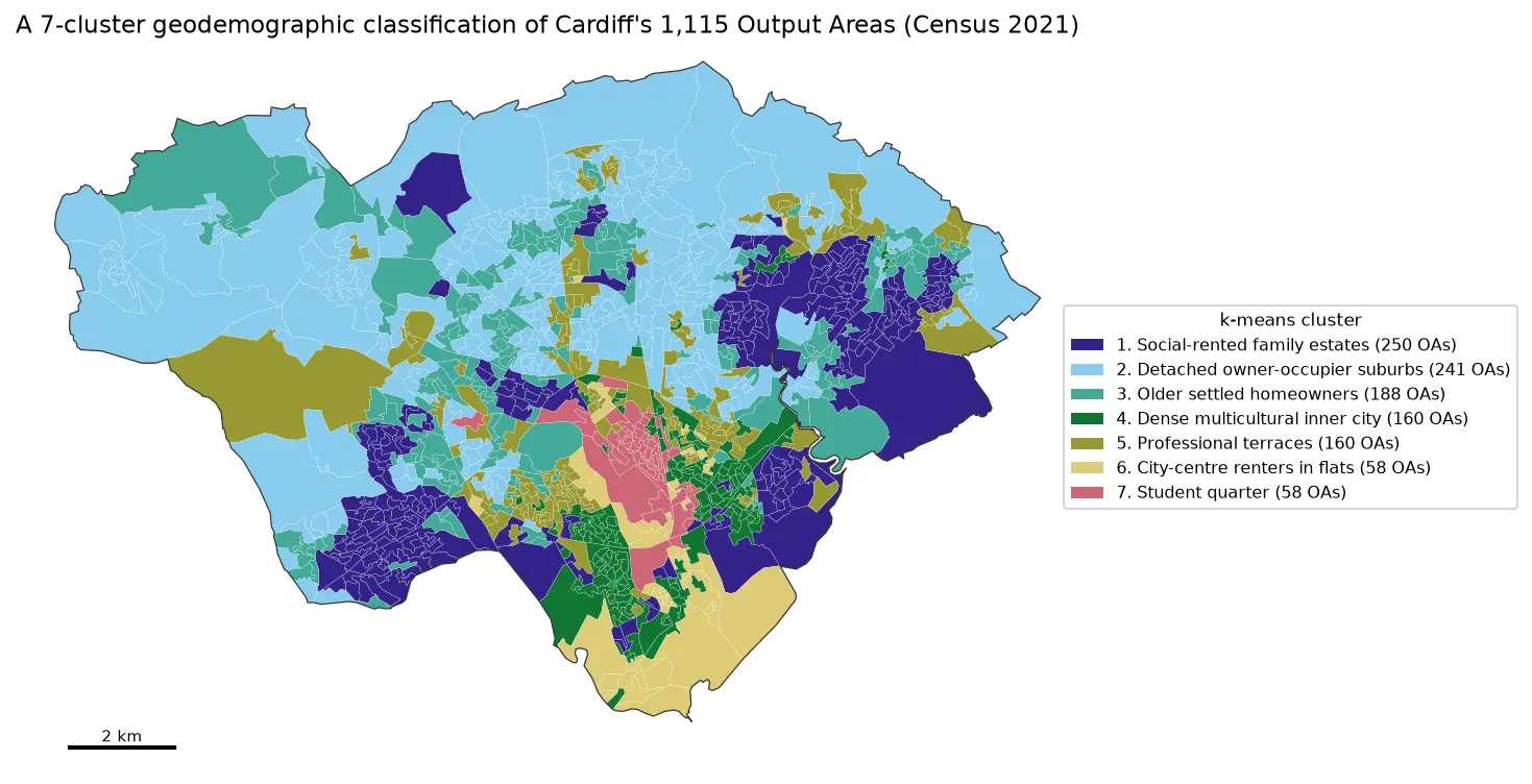
Geodemographic classification in Python: k-means on Census 2021 Output Areas, and SKATER and max-p regionalisation

Build a small geodemographic classification of Cardiff's 1,115 Census 2021 Output Areas in Python: choose and transform variables from Nomis bulk tables, standardise them, check correlations, choose k for k-means with the elbow, silhouette and stability across seeds, profile and cautiously name the clusters with index scores and radar charts, compare the result with the official 2021/2 OAC, test the MAUP at LSOA level, and contrast it with contiguous regions from spopt's SKATER and max-p.

Intermediate 17 min read

Tutorial Spatial Analysis Part 2 of 2

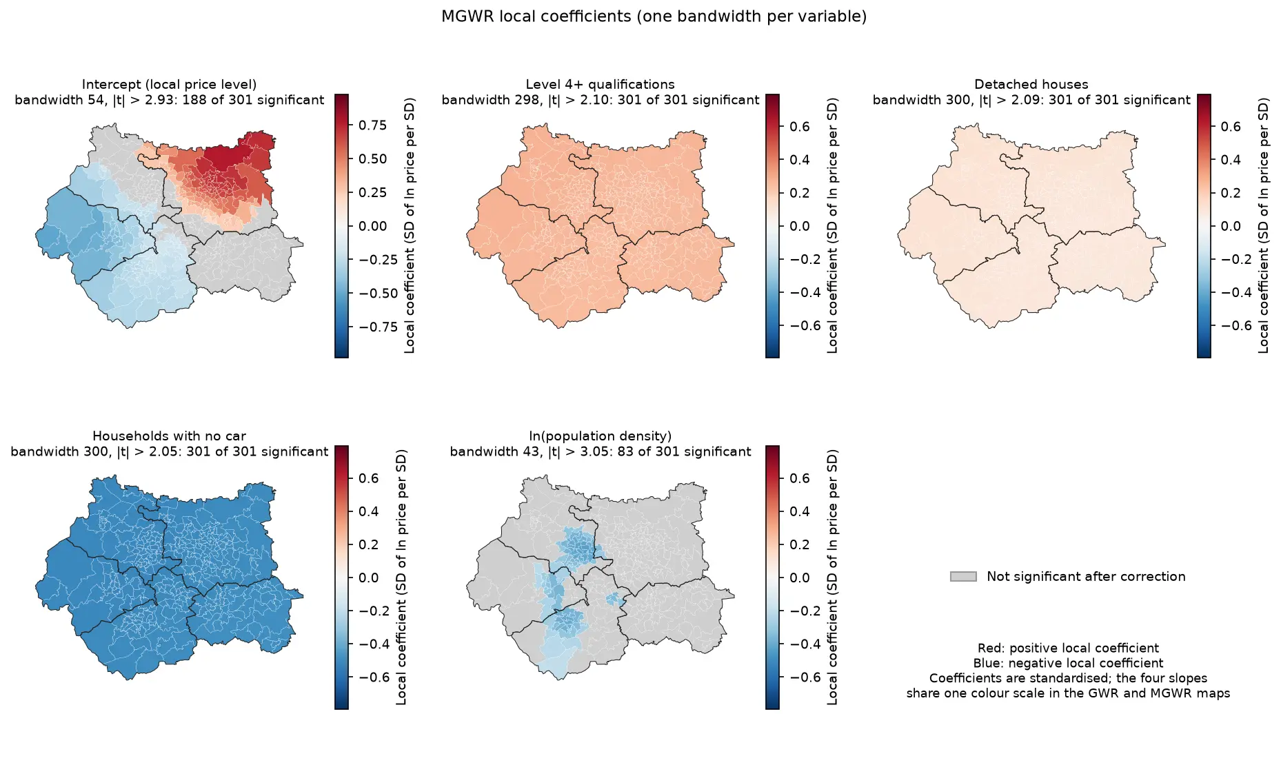
Geographically weighted regression in Python: GWR and MGWR with mgwr

Fit geographically weighted regression (GWR) and multiscale GWR (MGWR) in Python with the mgwr package on real West Yorkshire house prices: choose the bandwidth by AICc, map local coefficients with a multiple-testing correction, read local R² and local collinearity, and compare against global OLS, spatial lag and spatial error models.

Advanced 17 min read

Tutorial Python Part 2 of 2

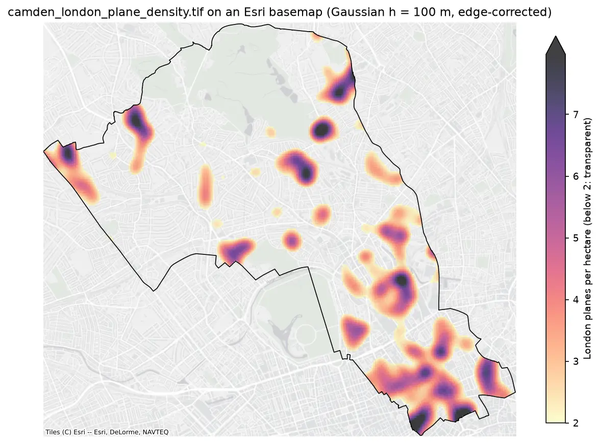
Kernel density estimation in Python for GIS: bandwidths, GeoTIFF heatmaps and relative risk

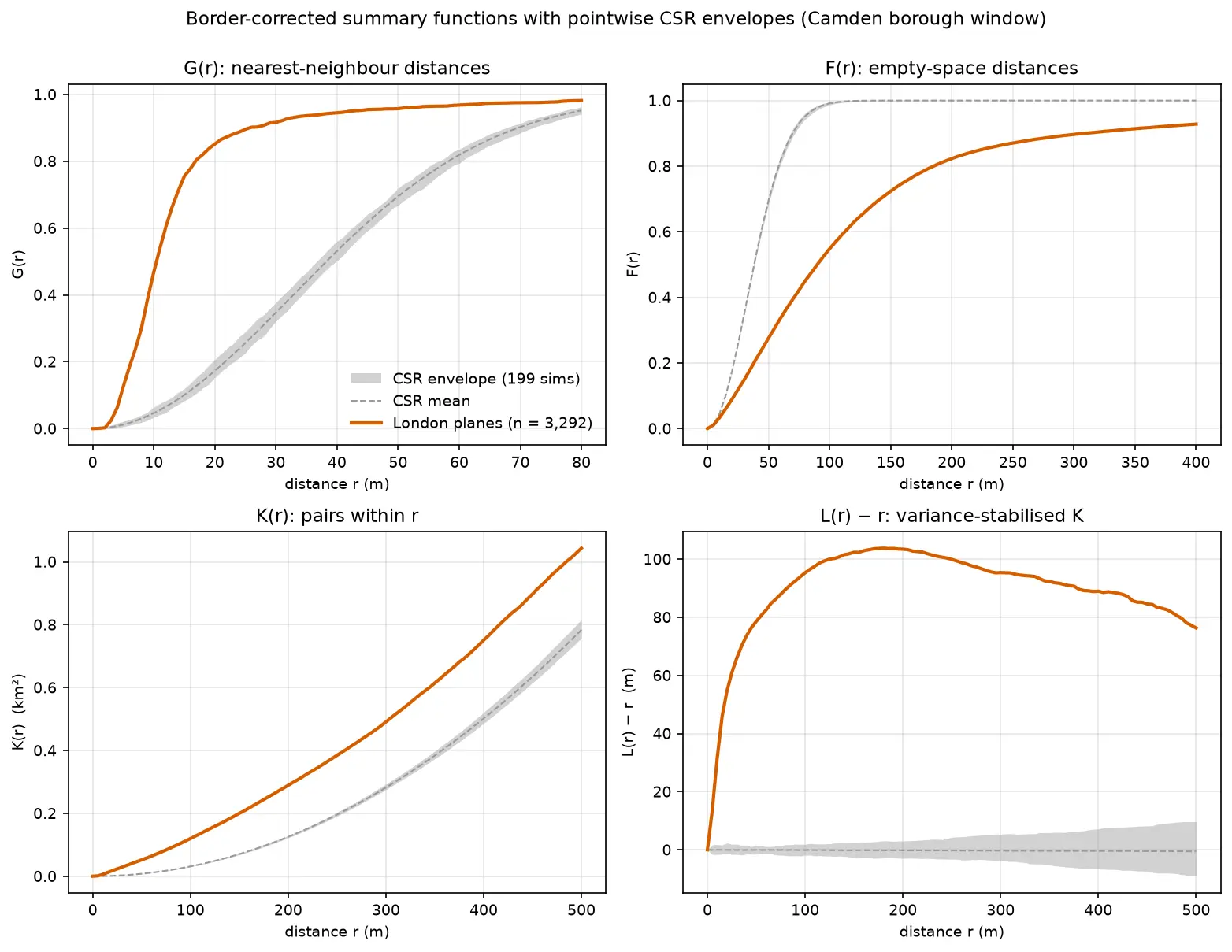
Make a kernel density heatmap from points in Python: compare Scott/Silverman, likelihood cross-validation and a fixed planning distance, Gaussian and Epanechnikov kernels and sample weights, export an edge-corrected GeoTIFF with rasterio, show it on a basemap, and map case-control relative risk on Camden's London plane trees.

Intermediate 16 min read

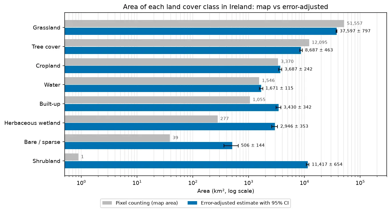
Bar chart comparing the area of each land cover class in Ireland from WorldCover pixel counting with the error-adjusted estimate and its 95% confidence interval.
Tutorial Remote Sensing

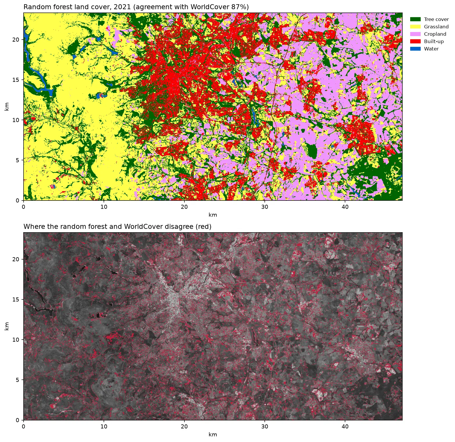
Land cover accuracy assessment in Python: confusion matrix, Olofsson area estimates and sample size

Assess a real land cover map in Python: ESA WorldCover 2021 against 8,597 Eurostat LUCAS 2022 field survey points in Ireland. Build the confusion matrix, compute overall, user's and producer's accuracy, see why kappa is discouraged, and use the Olofsson et al. (2014) stratified estimators to get error-adjusted areas with 95% confidence intervals and to plan a new stratified random sample.
Advanced 20 min read

Tutorial Python Part 2 of 2

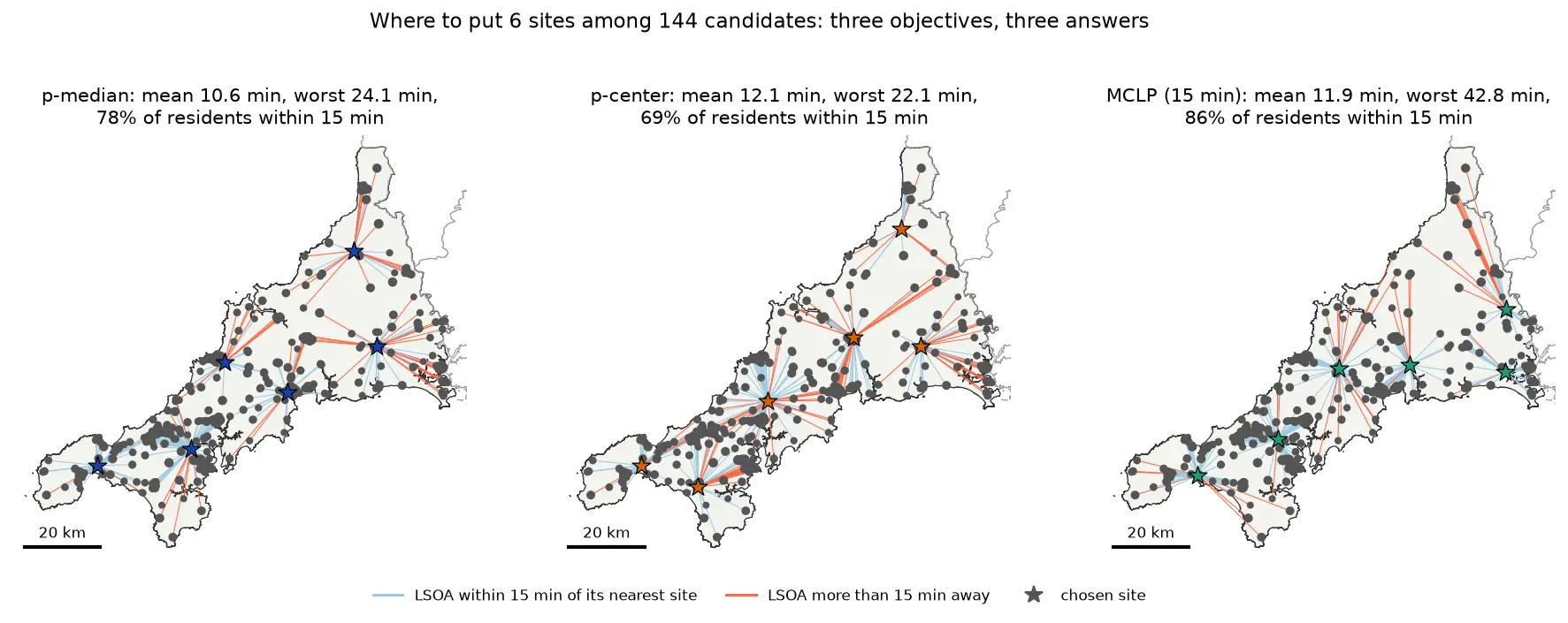
Location-allocation in Python: p-median, p-center and maximal covering (MCLP) with spopt

Solve location-allocation problems in Python with spopt and the CBC solver: the p-median, p-center and maximal covering location problem (MCLP). Choose sites for new urgent-care or mobile clinic bases among Cornwall's community buildings, on OSMnx drive times and Census 2021 population, compare the three answers on maps and charts, draw the trade-off curve as the number of sites grows, and see how problem size drives solve time.

Intermediate 17 min read

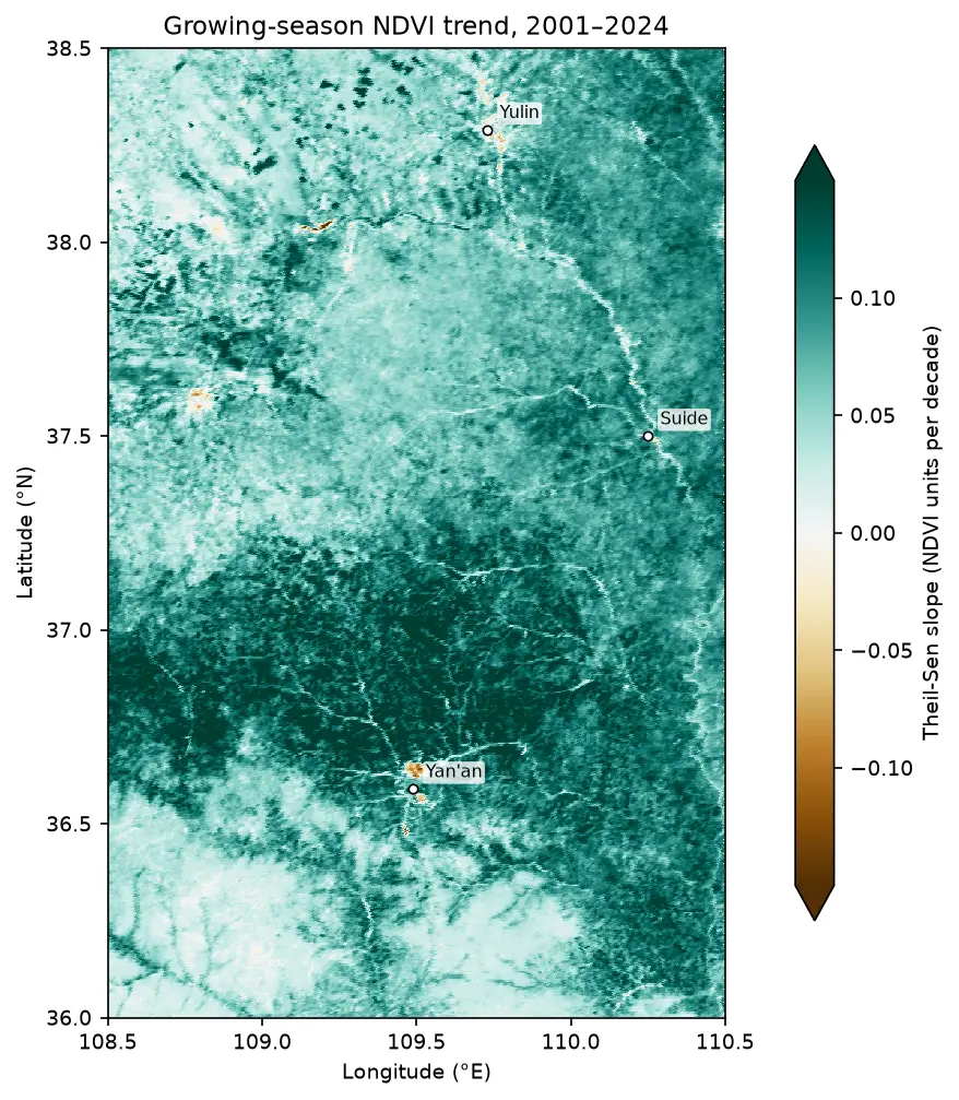
Map of the Theil-Sen slope of growing-season NDVI from 2001 to 2024 on the Loess Plateau between Yan'an and Yulin, almost entirely teal (greening), with a few brown browning patches near Yan'an and Yulin.

Tutorial Remote Sensing

Mann-Kendall trend test on rasters in Python: Theil-Sen NDVI trends with xarray

Run a pixel-wise Mann-Kendall trend test and Theil-Sen slope on 24 years of MODIS NDVI in Python. Read MOD13A1 from the Microsoft Planetary Computer, mask it with the QA layer, aggregate to growing-season means, vectorise the tests with xarray.apply_ufunc (checked against pymannkendall), compare the seasonal and modified Mann-Kendall tests, control the false discovery rate across 229,229 pixels, and map greening and browning on China's Loess Plateau.

Advanced 16 min read

Tutorial Python Part 1 of 2

Two-step floating catchment area (2SFCA) in Python: spatial access to GP practices in Cornwall

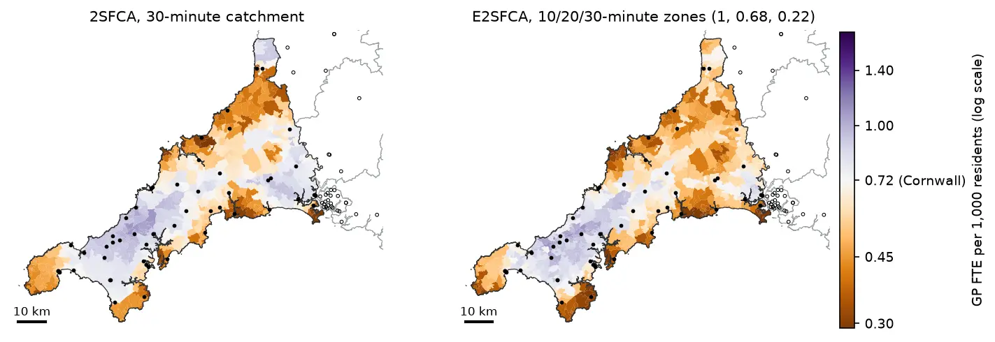
Measure spatial accessibility to GP practices in Python with the two-step floating catchment area (2SFCA) method and its distance-decay version (E2SFCA). Build OSMnx drive times for Cornwall from OpenStreetMap, use NHS GP workforce data and Census 2021 population, compare the PySAL access package with a vectorised NumPy version, and test the catchment threshold, the decay function and edge effects.

Intermediate 18 min read

Tutorial Spatial Analysis Part 1 of 2

Spatial regression in Python: OLS diagnostics, spatial lag and spatial error models with spreg

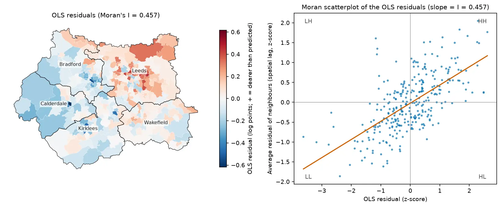
Fit spatial regression models in Python with PySAL's spreg on real West Yorkshire house prices: test the OLS residuals for spatial autocorrelation, read the Lagrange Multiplier diagnostics, fit spatial lag and spatial error models, compare them by AIC and log-likelihood, interpret direct, indirect and total impacts, and check how much the spatial weights matter.

Intermediate 18 min read

Tutorial Python

Methane plume detection in Python with NASA EMIT: mapping and quantifying landfill plumes

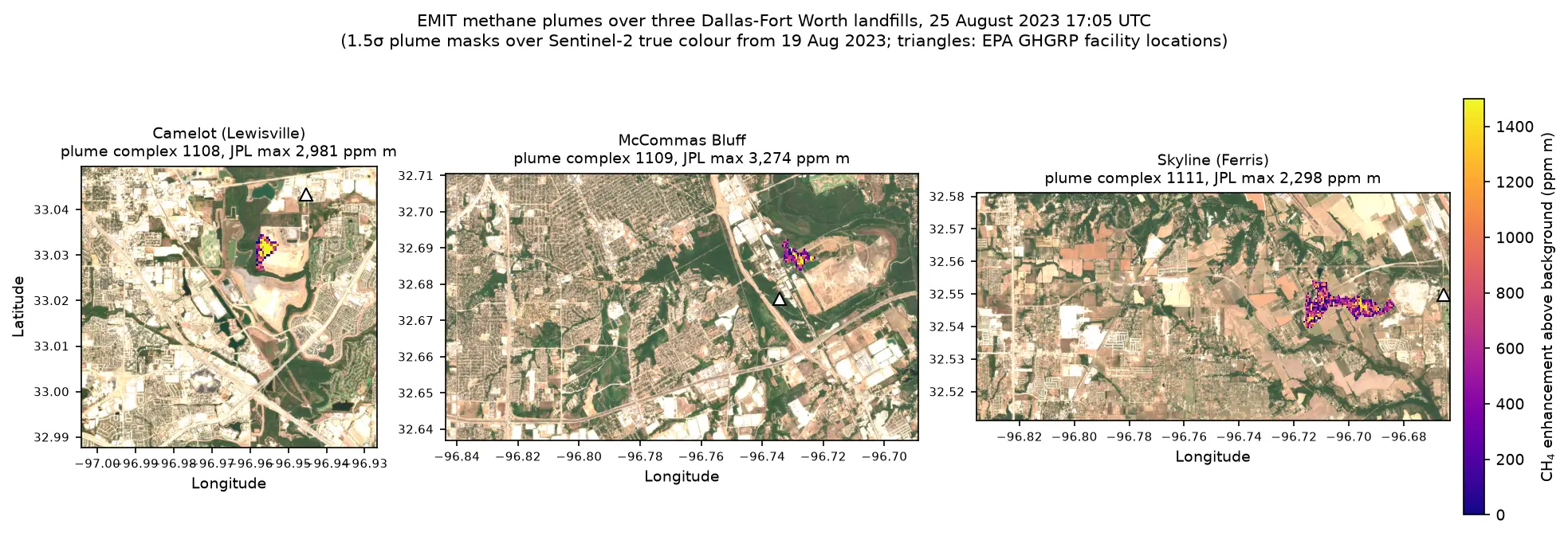
Detect and quantify methane plumes in Python with NASA's EMIT imaging spectrometer: load open EMIT methane enhancement data from NASA VEDA without a login, separate three Dallas-Fort Worth landfill plumes from the noise, compute the integrated mass enhancement, estimate emission rates with ERA5 winds, and compare them with EPA greenhouse gas inventory figures.

Advanced 17 min read

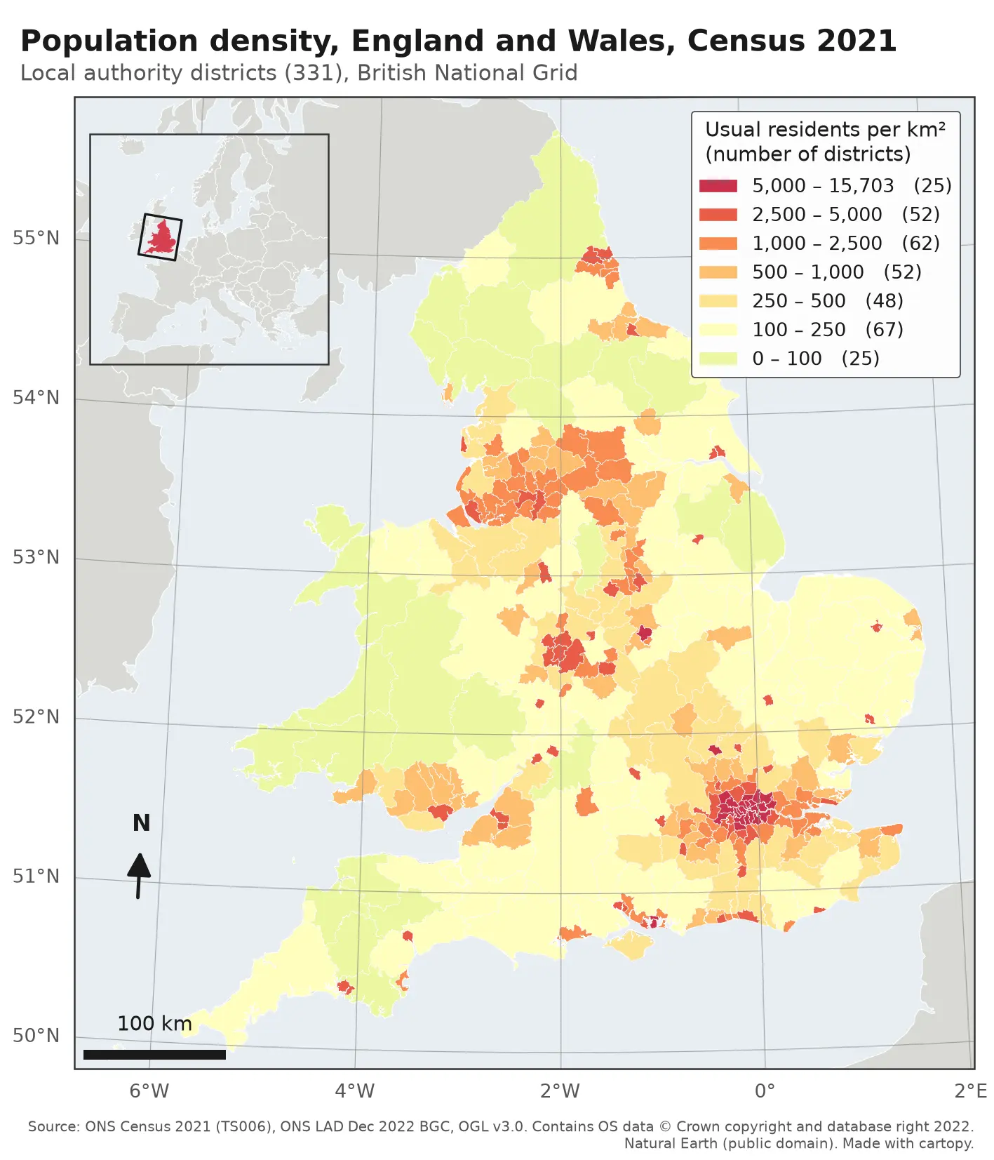
Choropleth map of population density in the 331 local authority districts of England and Wales from Census 2021, in seven classes from pale yellow (under 100 residents per km²) to deep red (over 5,000). London, Birmingham, Manchester, Liverpool, Leeds, Newcastle and the south coast cities stand out in red; Wales, Cumbria, Northumberland and Lincolnshire are pale. The map has a classified legend, a 100 km scale bar, a north arrow, latitude and longitude labels and an inset locator map of Europe.

Tutorial Python

Make a map in Python with matplotlib and cartopy: projections, classified choropleths, scale bars, north arrows and inset maps

A cartopy tutorial for publication-quality maps in Python: choose a projection, draw a classified choropleth of Census 2021 population density with a proper legend, add a scale bar, a true-north arrow, an inset locator map and gridlines, style it for light and dark backgrounds, export at 300 dpi to PNG, PDF and SVG, and shade the Copernicus DEM for Greater Manchester.

Beginner 14 min read

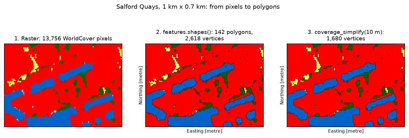
Three panels of the same 1 km by 0.7 km area at Salford Quays. Left: square WorldCover pixels, mostly red built-up land with blue dock basins and small green and yellow patches. Middle: the same area as 142 polygons with black outlines that follow the pixel staircase. Right: the polygons after coverage simplification at 10 m, with smoother outlines and no gaps between them.

Tutorial Python Part 3 of 3

Raster to vector in Python: polygonize with rasterio, rasterize boundaries and convert a GeoTIFF to a Cloud Optimized GeoTIFF

Convert raster to vector in Python with rasterio.features.shapes on 10 m ESA WorldCover for Greater Manchester: polygonize water and built-up land, fix invalid polygons, simplify without gaps, rasterize ONS district boundaries for land-cover shares, then write and validate a Cloud Optimized GeoTIFF with rio-cogeo and measure HTTP range reads.

Intermediate 14 min read

Tutorial Python

Rooftop solar potential from LiDAR in Python: pvlib, PVGIS and shading for every roof

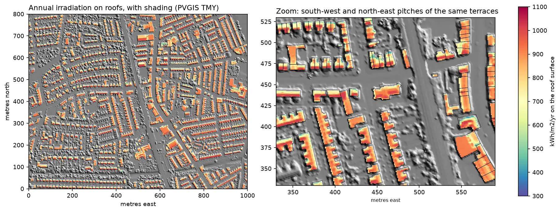
Estimate rooftop solar potential in Python for 2,148 buildings in Manchester: take a 1 m Environment Agency LiDAR DSM and Overture Maps footprints, compute roof slope and aspect, trace horizon angles for shading from neighbours and trees, build a sun map from a PVGIS typical year with pvlib, check it against pvlib's Perez model and PVGIS, then estimate kWp and kWh per year per roof and rank the best roofs.

Advanced 14 min read

Tutorial Python

Sentinel-1 soil moisture in Python: change detection checked against COSMOS-UK

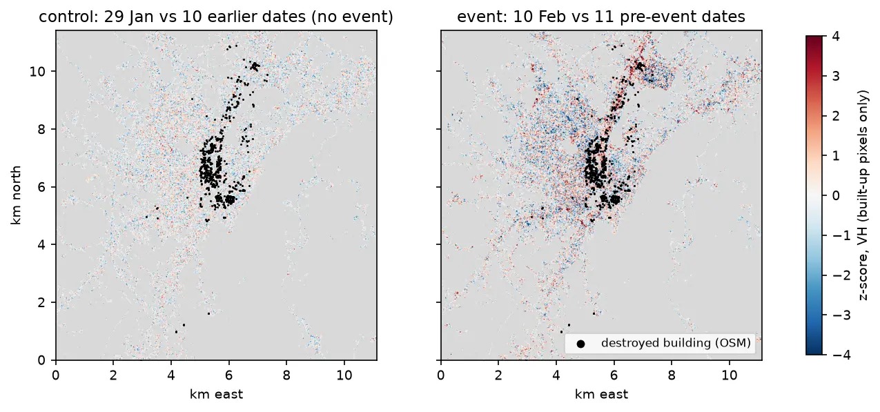
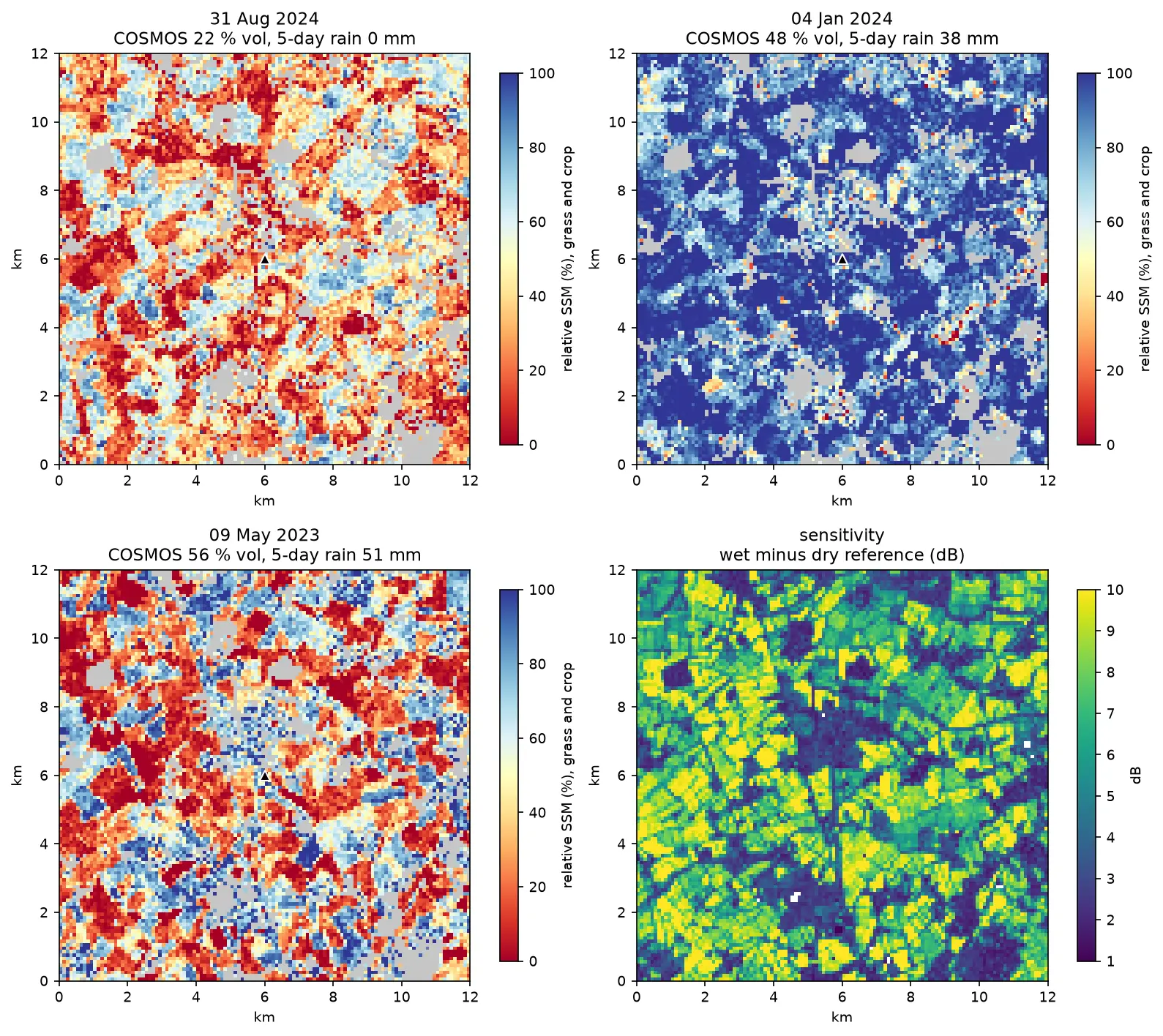
Estimate surface soil moisture from free Sentinel-1 radar in Python with the TU Wien change-detection method. Build dry and wet references per orbit, map relative soil moisture at 100 m, and test it honestly against four COSMOS-UK stations and their rain gauges.

Intermediate 13 min read

Tutorial Python Part 2 of 3

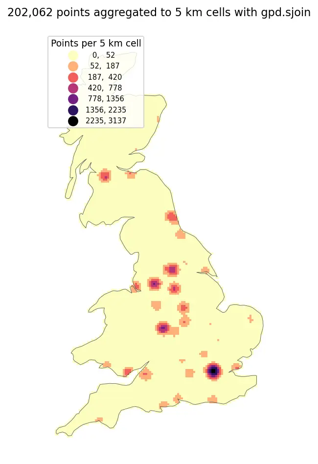
Spatial joins in GeoPandas: sjoin, predicates, sjoin_nearest and point in polygon

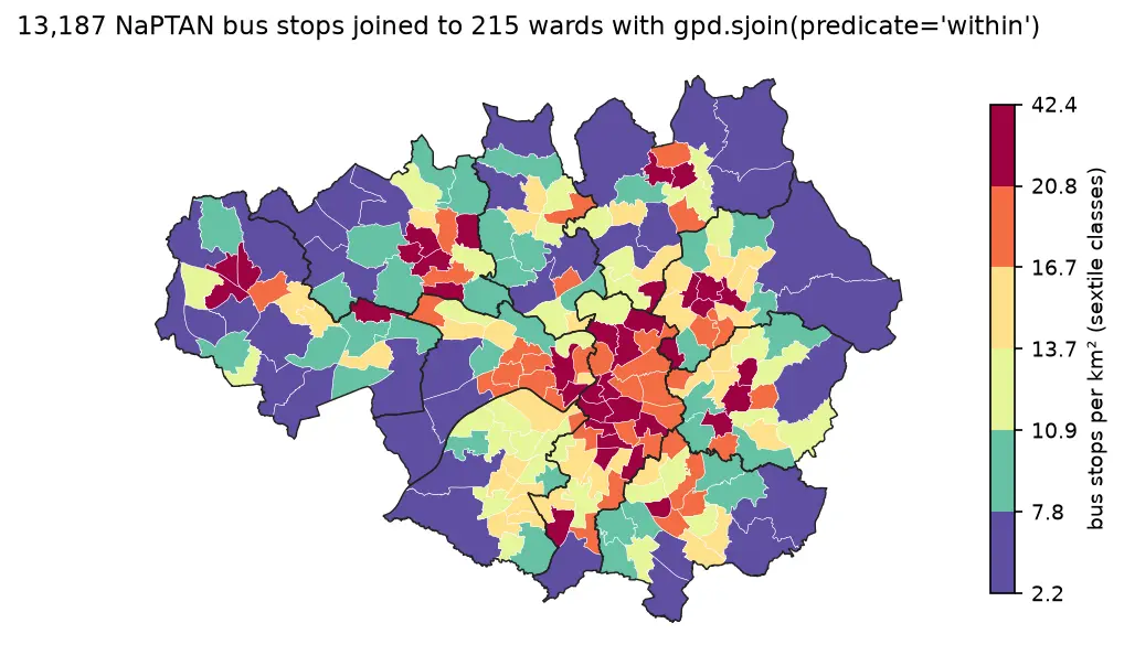
A practical guide to spatial joins in GeoPandas with real Greater Manchester data: 13,187 NaPTAN bus stops, 1,386 OpenStreetMap schools, 215 ONS wards and 1,702 LSOAs. Covers point in polygon with sjoin, predicates, counts per polygon, how='left'/'inner'/'right', sjoin_nearest with max_distance, clip and overlay, and a timing comparison of a naive loop against the spatial index.

Beginner 12 min read

Tutorial Python Part 1 of 3

Coordinate reference systems in Python: EPSG codes, pyproj transforms and reprojecting vectors and rasters

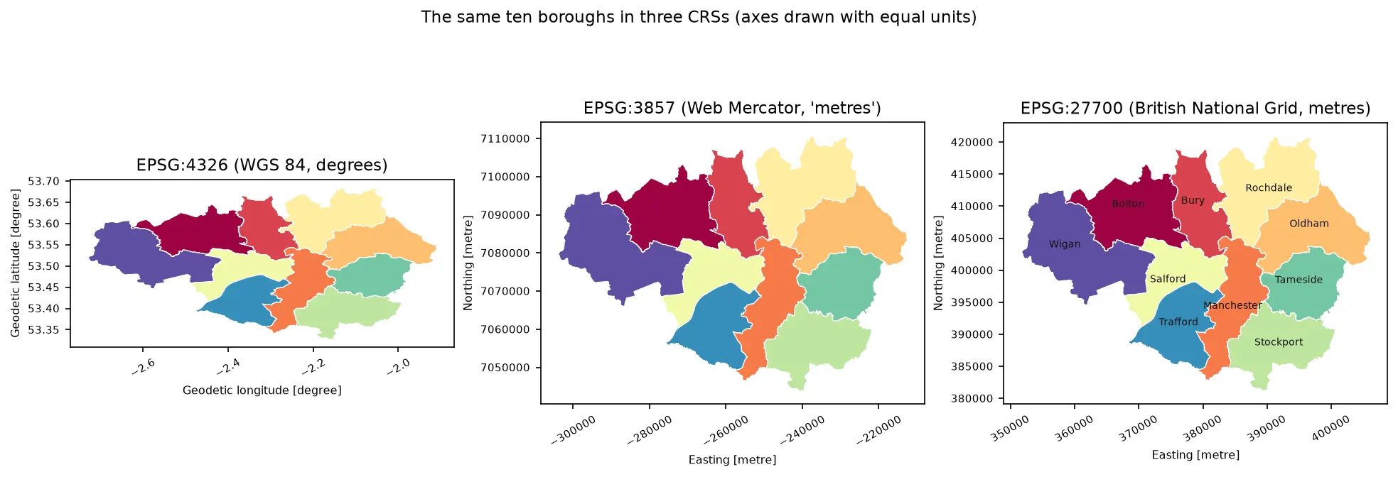
A practical guide to coordinate reference systems in Python with pyproj, GeoPandas and rasterio, tested on real Greater Manchester data. Covers EPSG codes, WGS 84 vs British National Grid (EPSG:27700), the always_xy axis-order trap, OSTN15 vs Helmert datum shifts checked against 13,187 NaPTAN bus stops, measured area and distance errors in the wrong CRS, and reprojecting a GeoDataFrame and a Copernicus DEM raster.

Beginner 13 min read

Tutorial Python

Viewshed analysis in Python: line of sight and a wind farm ZTV with GDAL and numpy

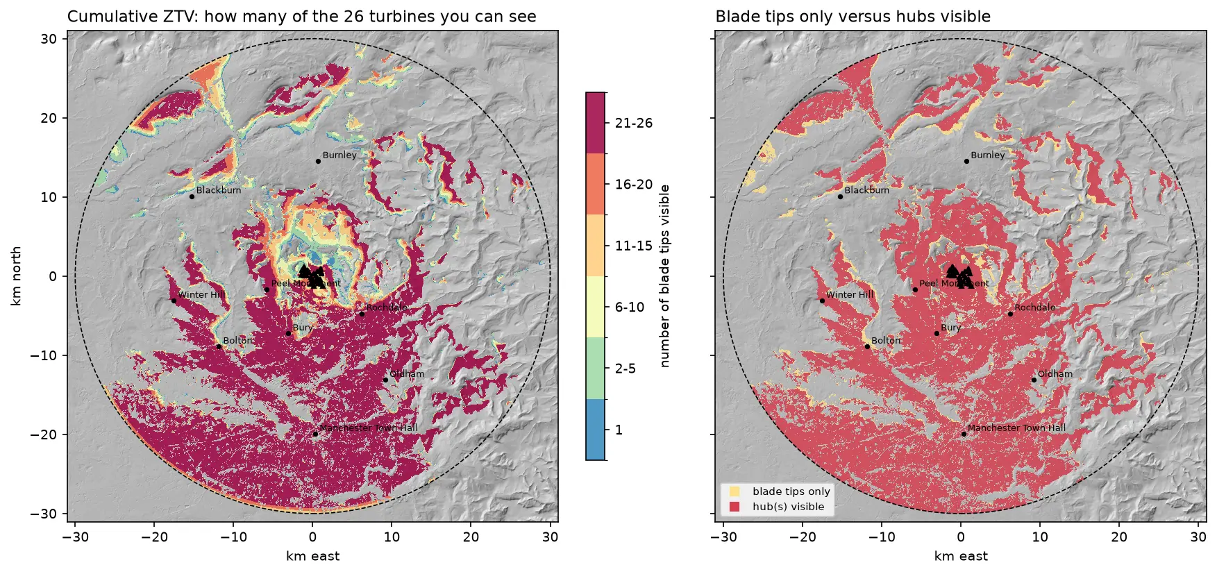
Run a viewshed analysis in Python on a real DEM: compute what one wind turbine can see with gdal.ViewshedGenerate, rebuild the same line-of-sight algorithm in numpy, correct for earth curvature and refraction, build a cumulative zone of theoretical visibility (ZTV) from 26 turbines, draw line-of-sight profiles, and measure how much trees and buildings in a LiDAR DSM shrink a bare-earth viewshed.

Intermediate 16 min read

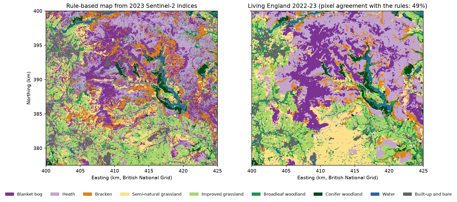
Two habitat maps of the Dark Peak side by side. Left: the rule-based map from Sentinel-2, with purple blanket bog and lilac heath on the Kinder and Bleaklow plateaux, orange bracken on the valley sides, green grassland and woodland in the valleys and blue reservoirs in the Derwent valley. Right: Living England 2022-23 for the same area, with smoother patches of the same classes.

Tutorial Python Part 1 of 5

Habitat mapping with Sentinel-2 in Python: spectral index rules and an honest accuracy assessment

Map blanket bog, heath, bracken, grassland, woodland, water and built-up land in the Peak District from 2023 Sentinel-2 seasonal composites with an eight-rule spectral index classifier, then assess it properly: a confusion matrix, user's and producer's accuracy, kappa and its caveats, block-bootstrap confidence intervals, and why a random train/test split overstates accuracy.

Beginner 19 min read

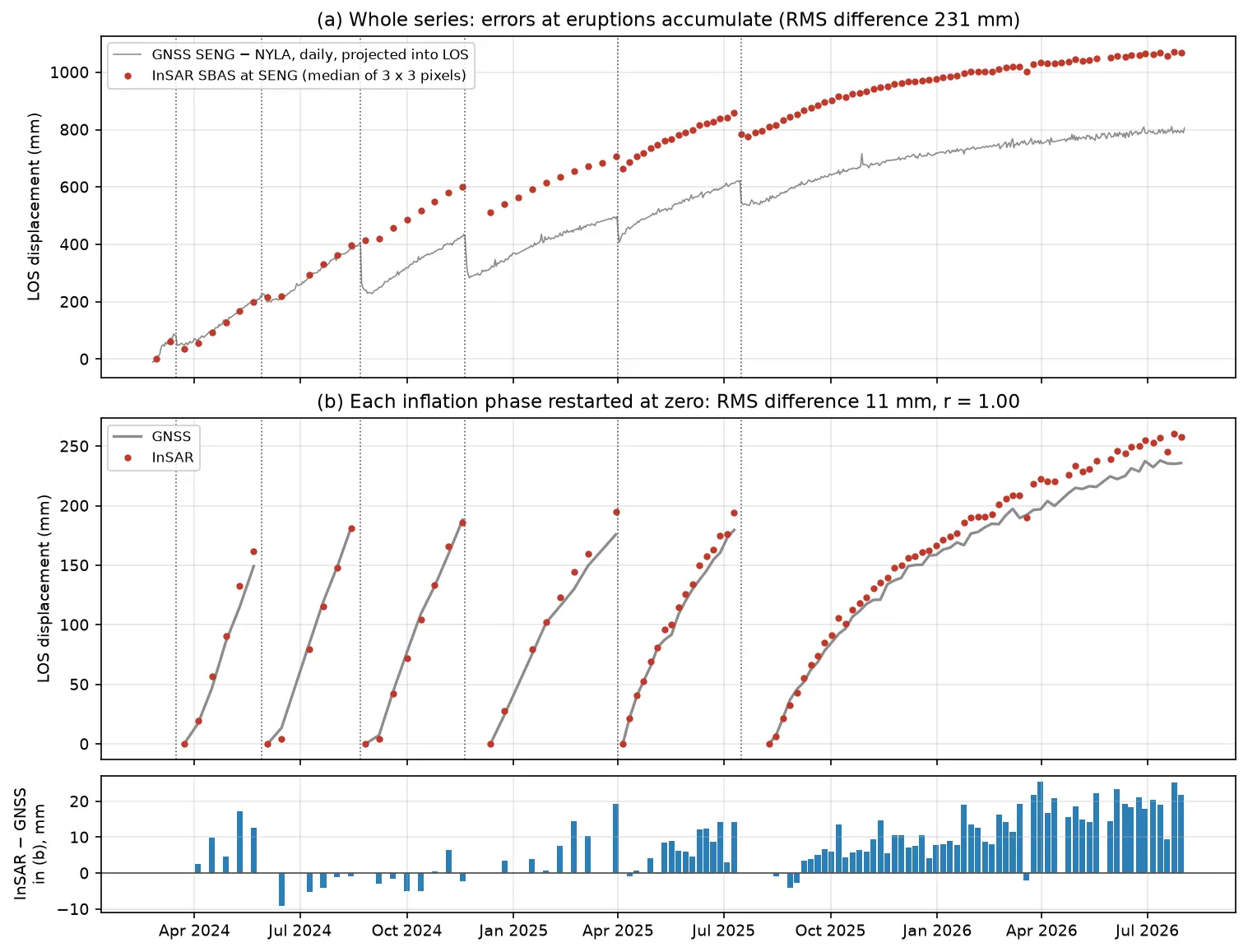
Time series of line-of-sight uplift at the SENG GNSS station at Svartsengi in Iceland from 2024 to 2026: red InSAR points and a grey GNSS line rise in a sawtooth of six inflation phases separated by eruptions, and agree closely once each phase is restarted at zero.

Tutorial Python Part 3 of 3

InSAR time series in Python: Svartsengi inflation cycles validated with GNSS

Build an SBAS InSAR time series in Python from 364 COMET LiCSAR Sentinel-1 interferograms of the Svartsengi volcano in Iceland. Check unwrapping with phase closure, invert pixel by pixel with weighted least squares, project GNSS east, north and up into the line of sight, and validate six inflation–eruption cycles against the SENG station.

Advanced 21 min read

Tutorial Python

Zonal statistics in Python: exactextract vs rasterstats, with partial pixels, land-cover fractions and a benchmark

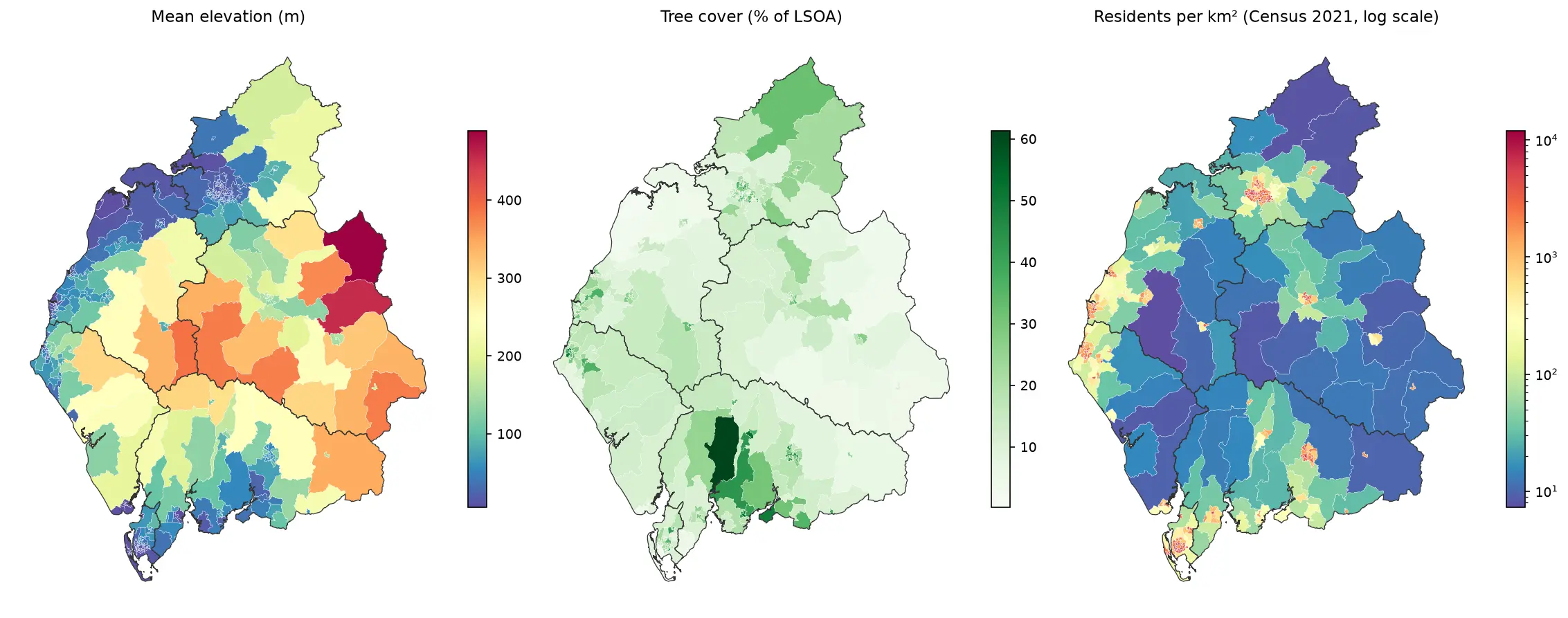
Calculate zonal statistics in Python with exactextract and rasterstats on real data: ONS 2021 LSOA boundaries for Cumbria with GHSL population, the Copernicus DEM and ESA WorldCover. Covers partial-pixel weighting vs pixel centroids, CRS alignment, categorical land-cover fractions, a speed benchmark, GeoPackage export and choropleth maps.

Intermediate 14 min read

Tutorial Python

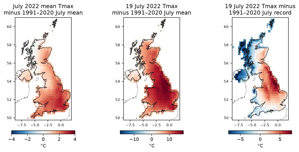
ERA5 in Python with xarray: mapping the July 2022 UK heatwave

Read ERA5 climate reanalysis in Python with xarray from free, login-free cloud Zarr stores, clip it to the UK, compute area-weighted means and anomalies against 1991–2020, export a Cloud Optimised GeoTIFF and check it against Met Office stations.

Intermediate 13 min read

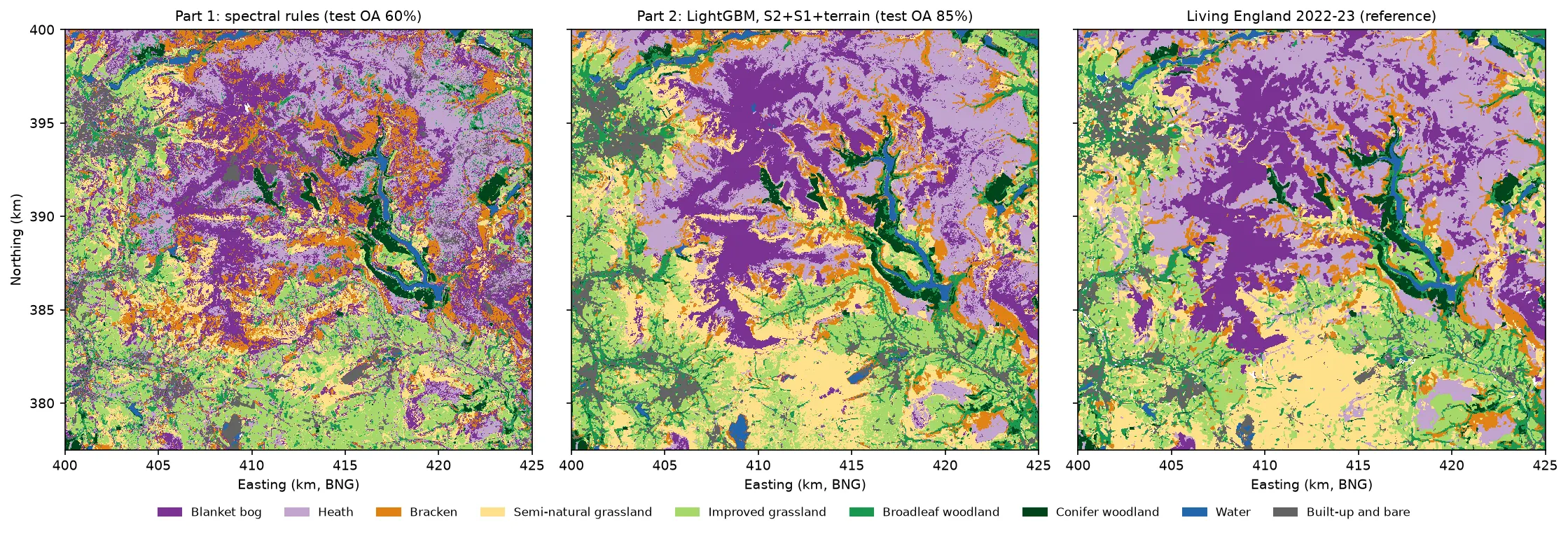
Three habitat maps of the Dark Peak side by side. Left: the noisy Part 1 rule-based map. Centre: the LightGBM map, with smooth purple blanket bog on the Kinder and Bleaklow plateaux, lilac heath around them, orange bracken on the valley sides, yellow semi-natural grassland in the south, green grassland and woodland in the valleys and blue reservoirs. Right: Living England 2022-23, which the LightGBM map closely resembles.

Tutorial Python Part 2 of 5

Habitat classification with LightGBM in Python: Sentinel-2, Sentinel-1 and terrain fusion

Classify nine upland habitats in the Peak District with LightGBM on 77 multi-temporal features: seasonal Sentinel-2 bands and indices, Sentinel-1 VV and VH backscatter and Copernicus DEM terrain. Tune with spatial-fold cross-validation and class weights, run an S2 / S2+S1 / S2+S1+terrain ablation, explain the model with TreeSHAP and permutation importance, and compare it with a random forest and the Part 1 rules on the same test blocks.

Intermediate 21 min read

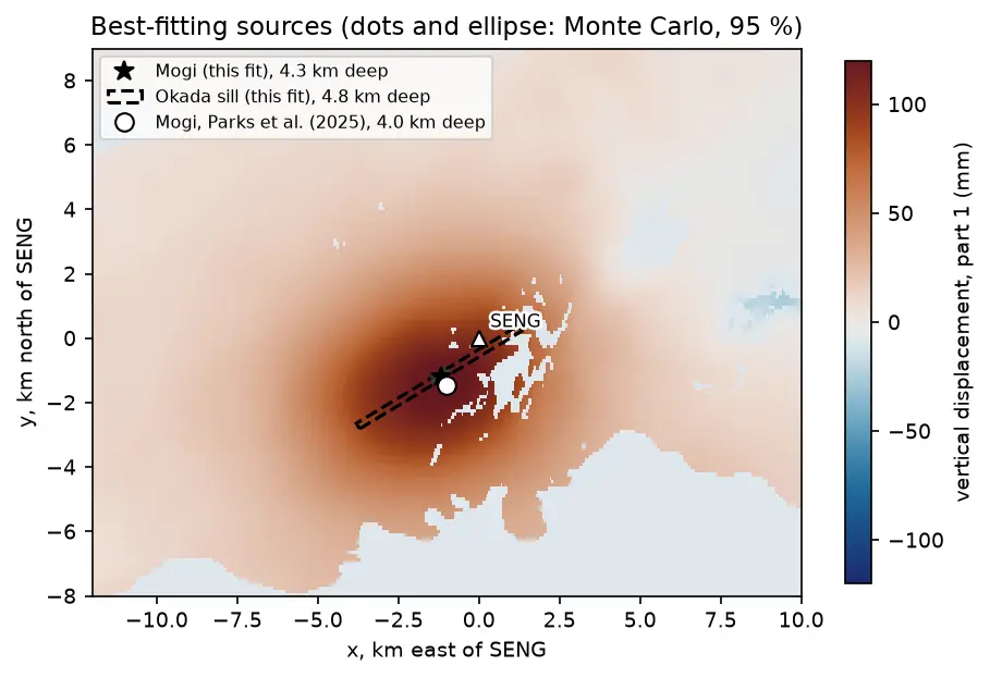
A map of vertical uplift at Svartsengi in Iceland with the best-fitting Mogi point source, an Okada sill outline and the published source location plotted near the centre of the uplift.

Tutorial Python Part 2 of 3

Mogi model inversion in Python: magma depth and volume from InSAR at Svartsengi, Iceland

Invert Sentinel-1 InSAR for a volcanic source in Python: write Mogi point-source and Okada (1985) sill forward models in NumPy, downsample ascending and descending LOS maps with a quadtree, fit depth and volume change by weighted least squares with scipy.optimize, and estimate uncertainties with a Monte Carlo of correlated noise, compared with published results.

Advanced 17 min read

Tutorial Python

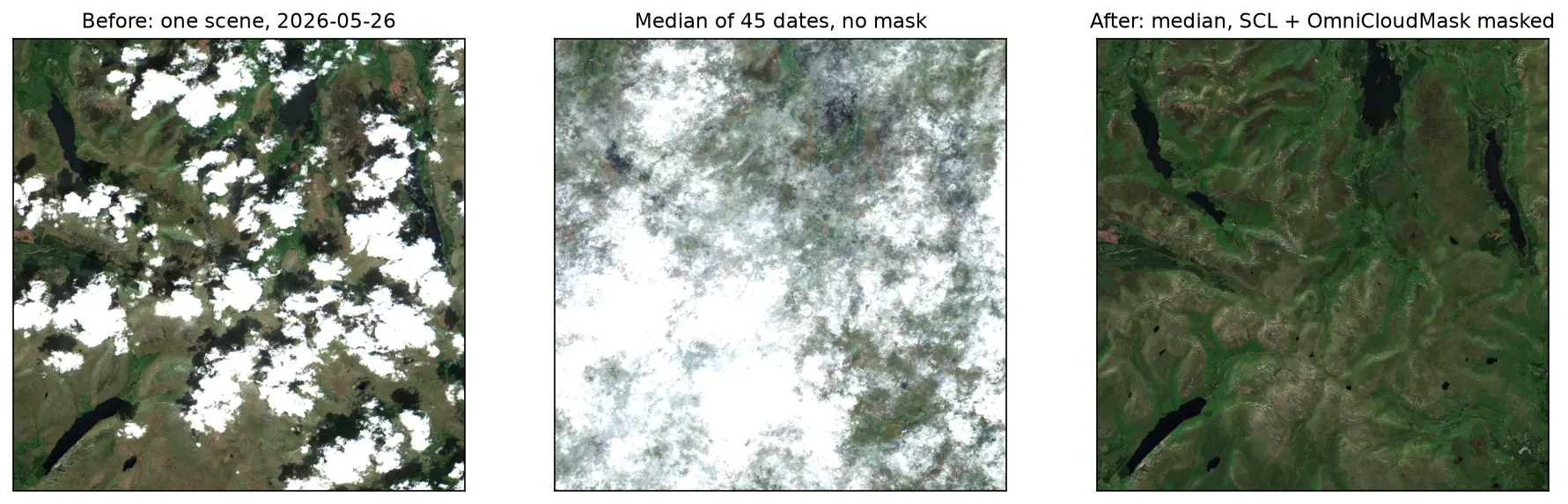
Sentinel-2 cloud and cloud-shadow masking in Python: SCL vs s2cloudless vs OmniCloudMask

Mask clouds and cloud shadows in Sentinel-2 L2A imagery with Python. Compare the Scene Classification Layer (SCL), s2cloudless, OmniCloudMask and a simple threshold over the Lake District, measure how far they agree, score them against 186 reference points and build a cloud-free median composite.

Intermediate 15 min read

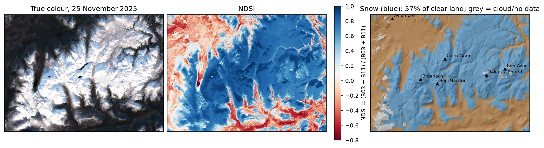
Three panels of the Cairngorms on 25 November 2025: a true-colour Sentinel-2 image with snow on the plateaux and long shadows in the glens; the NDSI, blue over snow and red over forest and bare ground; and a snow map over hillshade, with snow in blue on the high ground around Cairn Gorm, Ben Macdui, Braeriach, Beinn a' Bhuird and Ben Avon, covering 57% of the clear land.

Tutorial Python

Snow cover mapping with NDSI in Python: Sentinel-2 and MODIS over the Cairngorms

Map snow cover in Python with the Normalised Difference Snow Index (NDSI) from Sentinel-2 and the daily MODIS snow product on the Microsoft Planetary Computer: choosing the NDSI threshold, separating snow from cloud, snow-covered area through the winter of 2025–26 in the Cairngorms, and the snowline by elevation and aspect with the Copernicus DEM.

Intermediate 15 min read

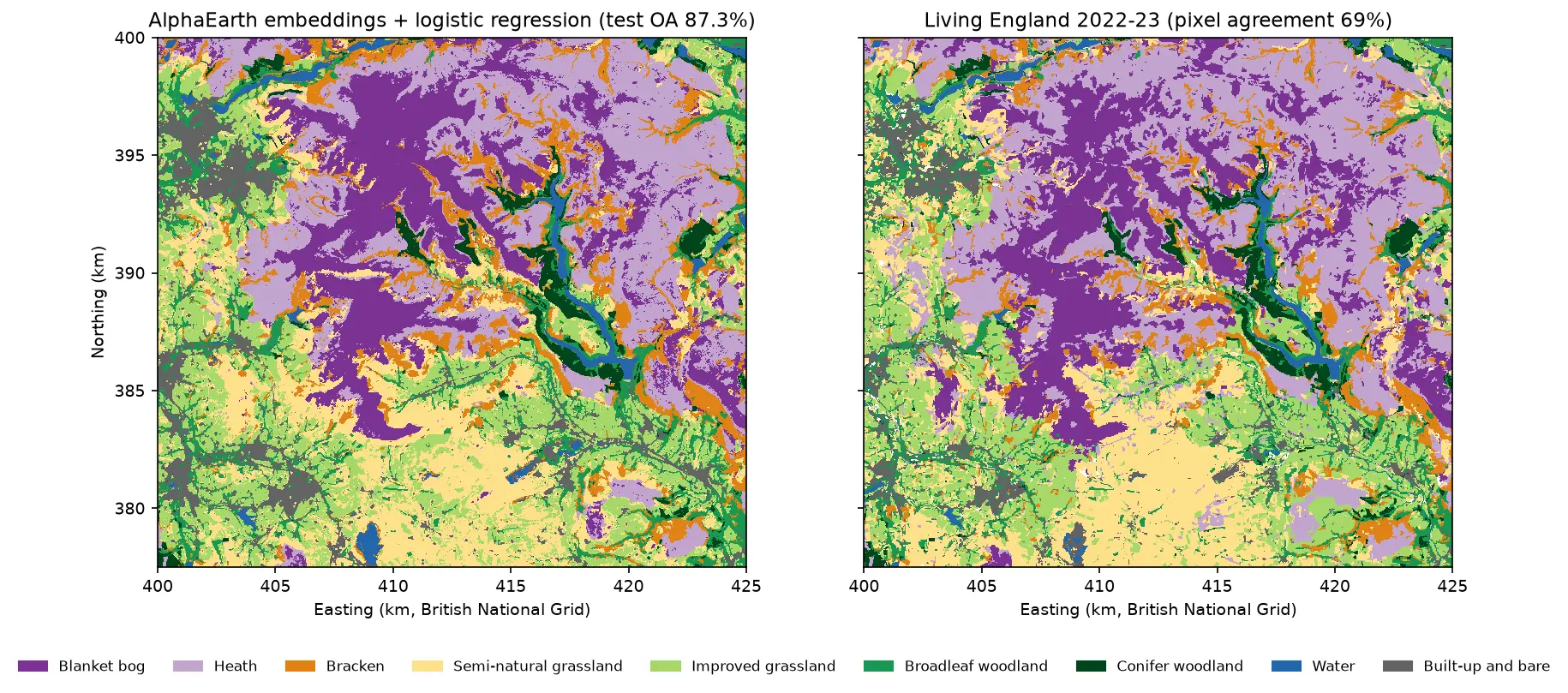
Two habitat maps of the Dark Peak side by side. Left: the map from AlphaEarth embeddings and logistic regression, with large purple blanket bog areas on Kinder Scout and Bleaklow, lilac heath around them, orange bracken on the valley sides, yellow and light green grassland in the south and west, and blue reservoirs in the Derwent valley. Right: Living England 2022-23 for the same area, with very similar patterns.

Tutorial Python Part 5 of 5

AlphaEarth satellite embeddings in Python: few-shot habitat mapping, uncertainty and area estimates

Use Google DeepMind's AlphaEarth Foundations satellite embeddings, a geospatial foundation model, in Python without a login. Classify nine Peak District habitats with a linear model, compare a few-shot learning curve against raw Sentinel-2 bands, map uncertainty, check calibration, simulate active learning, and estimate habitat areas with confidence intervals from a stratified random sample (Olofsson et al. 2014).

Advanced 24 min read

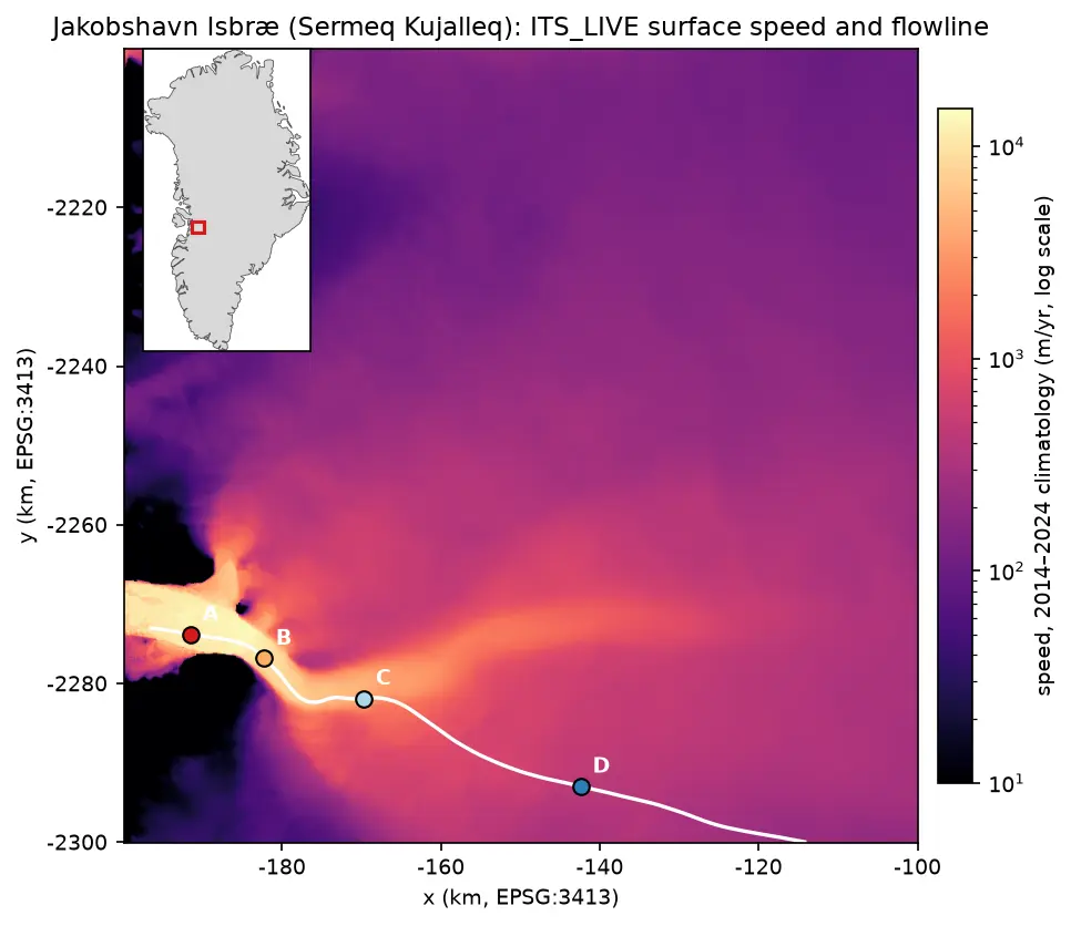
Map of ITS_LIVE surface speed around Jakobshavn Isbræ on a logarithmic colour scale: a narrow channel of ice faster than 10 km per year runs west into the fjord, fed by a broad fan of slower ice from the ice sheet. A white flowline runs up the trunk with points A to D marked at 5, 15, 30 and 60 km, and an inset shows the location on the west coast of Greenland.

Tutorial Python

Glacier velocity in Python with NASA ITS_LIVE: Jakobshavn Isbræ, 1985–2025

Map glacier velocity in Python with NASA's ITS_LIVE Zarr datacubes on AWS, with no login: velocity maps, a flowline traced from the velocity field, 40 years of speed profiles, seasonal and multi-year time series from 80,568 filtered image pairs, and strain rates and flow directions on Jakobshavn Isbræ (Sermeq Kujalleq), Greenland's fastest glacier.

Advanced 15 min read

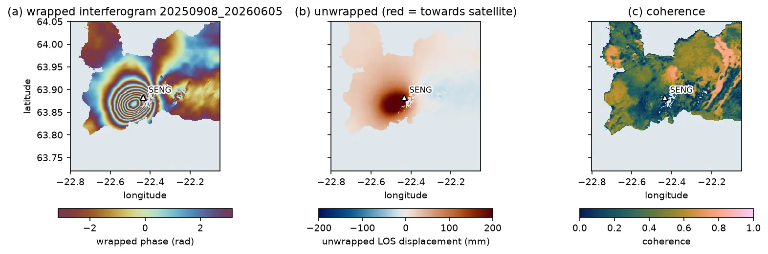
A Sentinel-1 interferogram of the Reykjanes Peninsula in Iceland with a bullseye of concentric colour fringes centred just west of the Svartsengi GNSS station, beside the unwrapped displacement and coherence maps.

Tutorial Python Part 1 of 3

InSAR volcano deformation in Python: mapping magma inflation at Svartsengi, Iceland, with Sentinel-1

Map volcano deformation with Sentinel-1 InSAR in Python: stream free COMET LiCSAR interferograms of the Svartsengi volcanic system in Iceland, read wrapped and unwrapped phase and coherence, count fringes, convert phase to line-of-sight millimetres, and combine ascending and descending tracks into vertical and east–west motion, checked against GNSS.

Advanced 19 min read

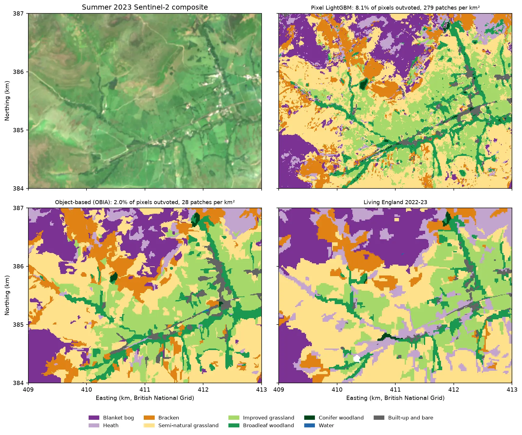
Four panels of the same 4 by 3 km area of the Edale valley and the southern edge of Kinder Scout. Top left: a true colour Sentinel-2 image of green fields and brown moorland. Top right: a pixel-based habitat map speckled with isolated pixels of other classes. Bottom left: the object-based map, with the same habitats in clean patches that follow field boundaries. Bottom right: the Living England reference map.

Tutorial Python Part 3 of 5

Object-based image analysis in Python: OBIA habitat classification with Sentinel-2

Segment 2023 Sentinel-2 seasonal composites of the Peak District into image objects with scikit-image SLIC and Felzenszwalb, tune the segment size against Living England boundaries, compute per-object statistics, shape and GLCM texture with NumPy, classify the objects with LightGBM and compare OBIA with a pixel-based classifier on accuracy, salt-and-pepper noise and patch counts. Then export the habitat objects as GeoPackage polygons.

Advanced 21 min read

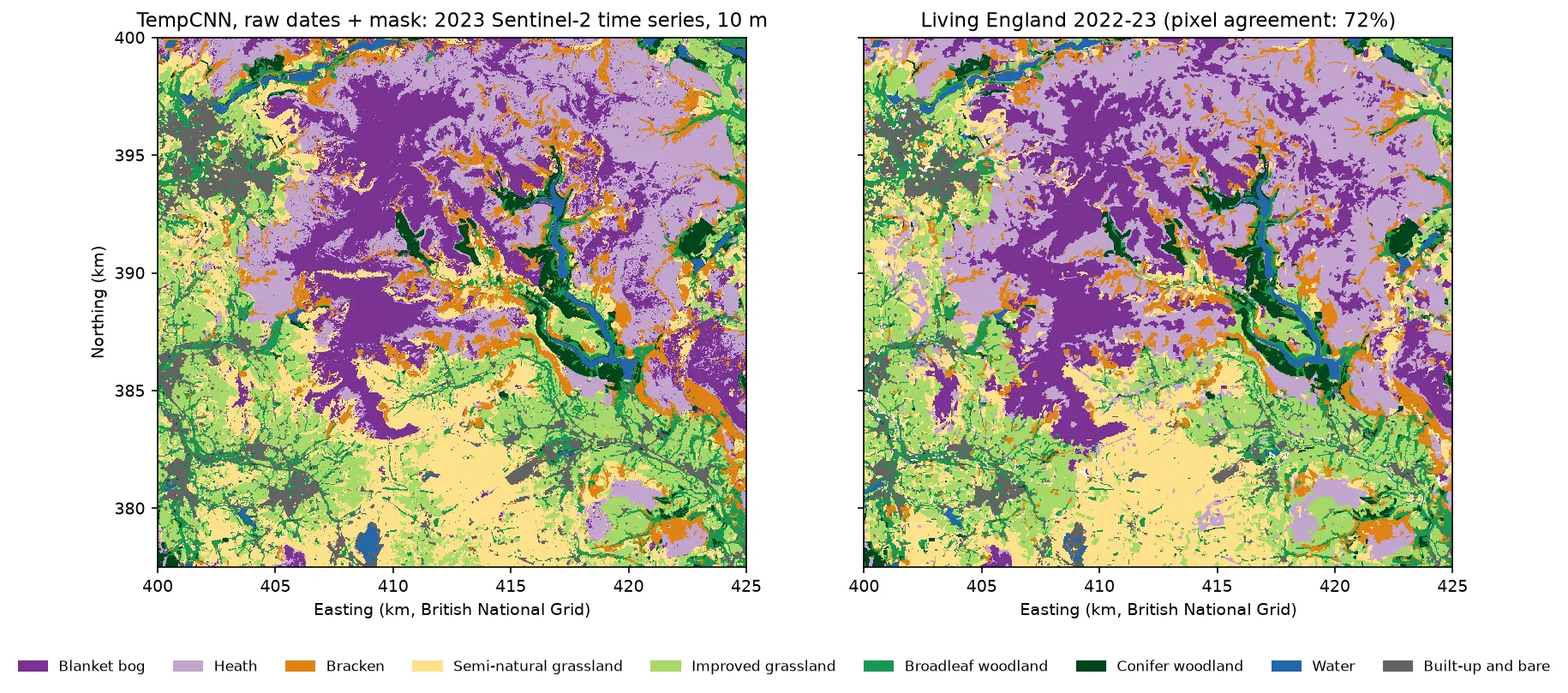
Two habitat maps of the Dark Peak side by side. Left: the TempCNN time-series map at 10 m, with purple blanket bog on the Kinder and Bleaklow plateaux, lilac heath around it, orange bracken on valley sides, yellow and green grassland in the south and west, dark green conifers and blue reservoirs in the Derwent valley. Right: Living England 2022-23 for the same area, which looks very similar but has more heath.

Tutorial Python Part 4 of 5

Satellite image time series classification with deep learning: TempCNN and L-TAE in PyTorch on a CPU

Classify habitats from a full year of cloudy, irregular Sentinel-2 observations with two temporal neural networks in PyTorch: a 1D convolutional TempCNN and a lightweight temporal attention encoder (L-TAE) with day-of-year positional encoding. Compare masking with gap-filling, test against a LightGBM baseline on spatial blocks, read which dates matter from attention and occlusion, and predict a wall-to-wall 10 m map on a CPU.

Advanced 24 min read

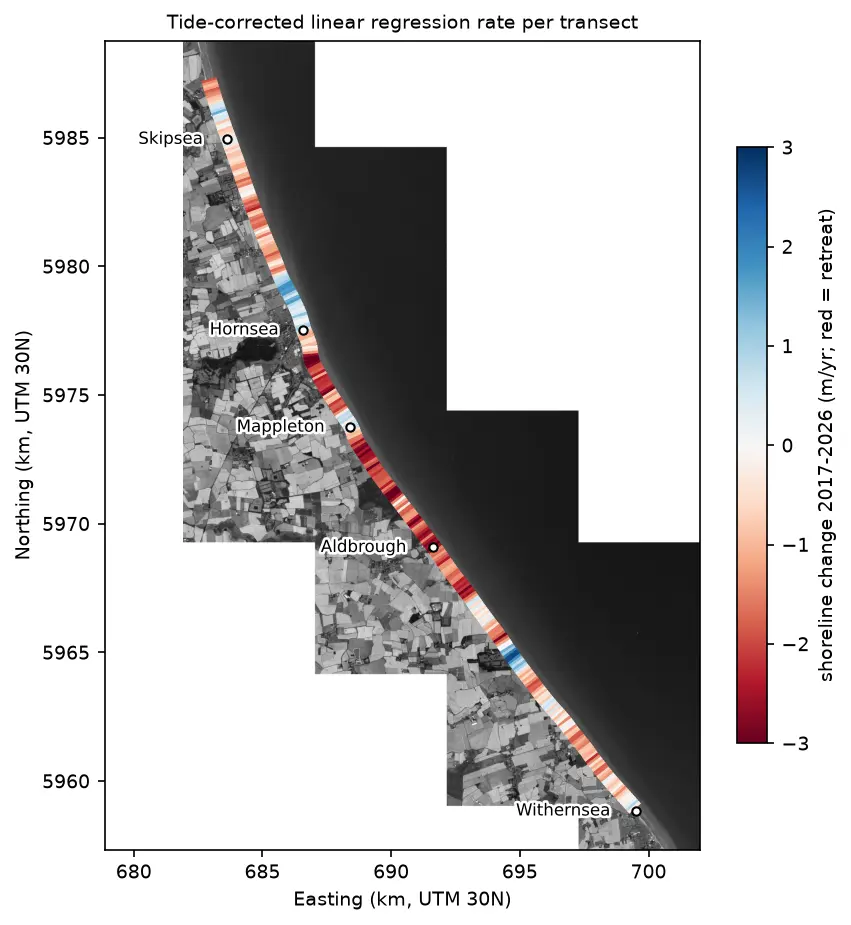
Map of the Holderness coast from Skipsea to Withernsea in greyscale Sentinel-2, with each 100 m transect coloured by its shoreline change rate from 2017 to 2026: mostly red (retreat), with blue (advance) patches north of Hornsea, at Mappleton and near Grimston.

Tutorial Python

Coastal erosion and shoreline change from Sentinel-2 in Python (Holderness, 2017–2026)

Measure shoreline change on one of Europe's fastest-eroding coasts with free Sentinel-2 imagery and Python: MNDWI and Otsu thresholding, sub-pixel shorelines with find_contours, shore-normal transects, a tide correction from open tide-gauge data, end-point and linear regression rates, and an honest comparison with East Riding of Yorkshire Council's cliff monitoring.

Advanced 21 min read

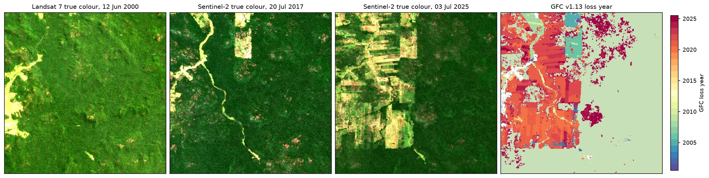
Tutorial Python

Deforestation detection in Python with Global Forest Change data (Rondônia, 2001–2025)

Map forest loss and deforestation in Python with the Hansen/UMD Global Forest Change v1.13 data: read the open tiles with no login, compute loss by year in hectares with correct pixel areas, compare Landsat and Sentinel-2 images before and after, and check the GFC loss year against Sentinel-2 NBR and MODIS burned area for central Rondônia, Brazil.

Intermediate 15 min read

Tutorial Python

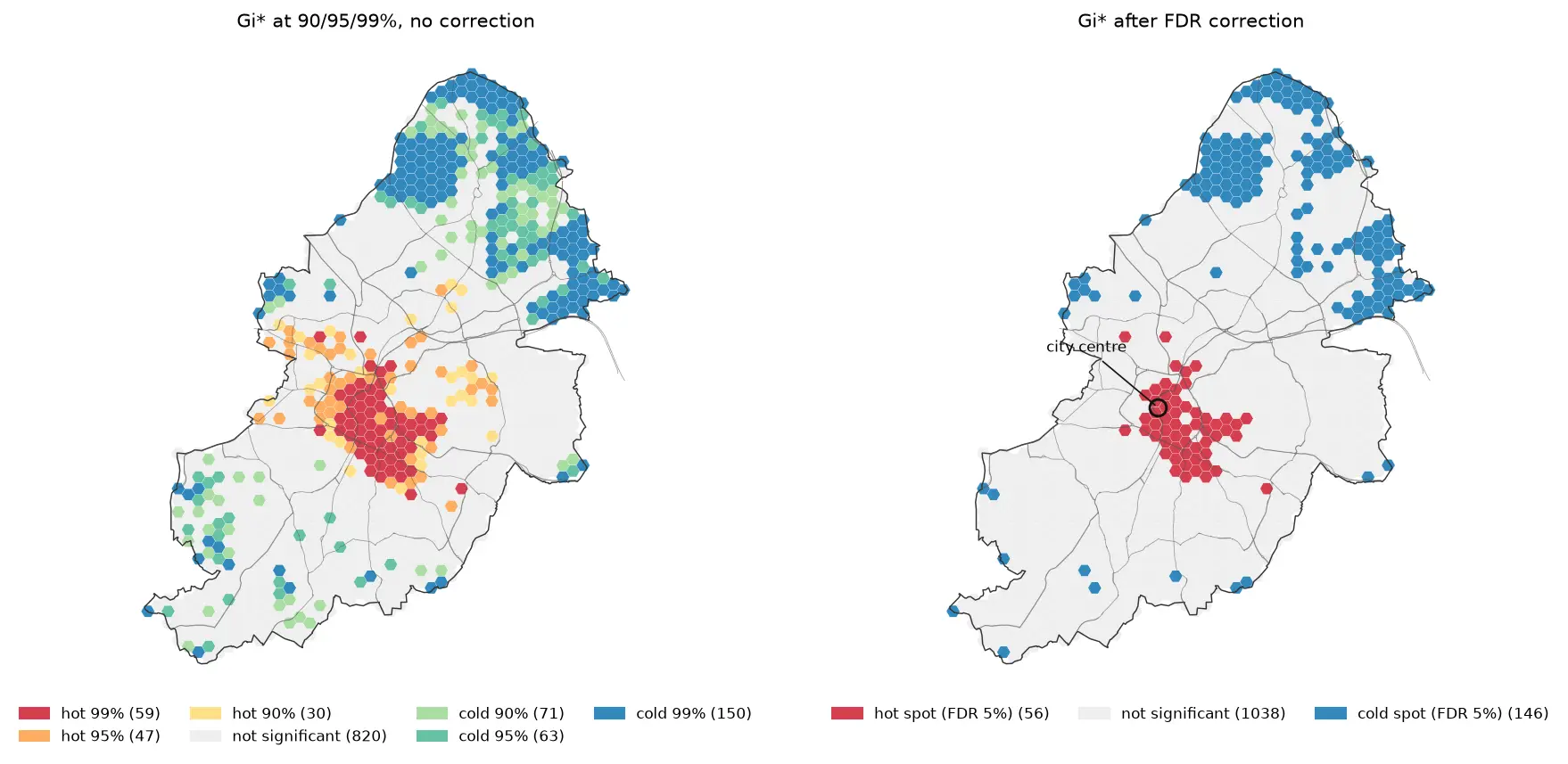
Hot spot analysis in Python: Getis-Ord Gi*, Moran's I and LISA on Birmingham road collisions

Run a hot spot analysis in Python with PySAL: aggregate 2025 STATS19 road collisions in Birmingham to a hexagon grid, test for clustering with global Moran's I, map Getis-Ord Gi* hot spots and LISA clusters with permutation inference and FDR correction, and see how spatial weights, the areal unit and exposure change the answer.

Intermediate 19 min read

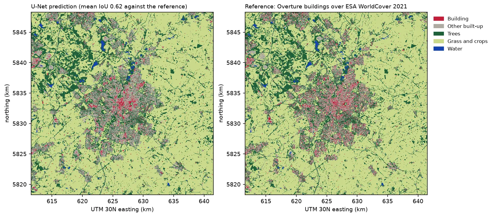
Two land cover maps of a 30 km square around Leicester side by side: the U-Net prediction on the left and the reference labels on the right. Both show the city in grey and red in the centre, surrounded by farmland in pale green, woods in dark green and reservoirs in blue. The prediction's city is smoother, with fewer separate red buildings.

Tutorial Python Part 3 of 3

Deep learning inference on large rasters: sliding-window prediction, COGs and polygons in Python

Run a trained PyTorch U-Net over a whole Sentinel-2 scene of a city it has never seen: tiled sliding-window inference on a large GeoTIFF with overlapping, blended windows, a georeferenced Cloud Optimised GeoTIFF of classes and confidence, raster-to-vector polygons with rasterio.features.shapes in a GeoPackage, and an honest check against reference labels.

Advanced 13 min read

Tutorial Python Part 2 of 2

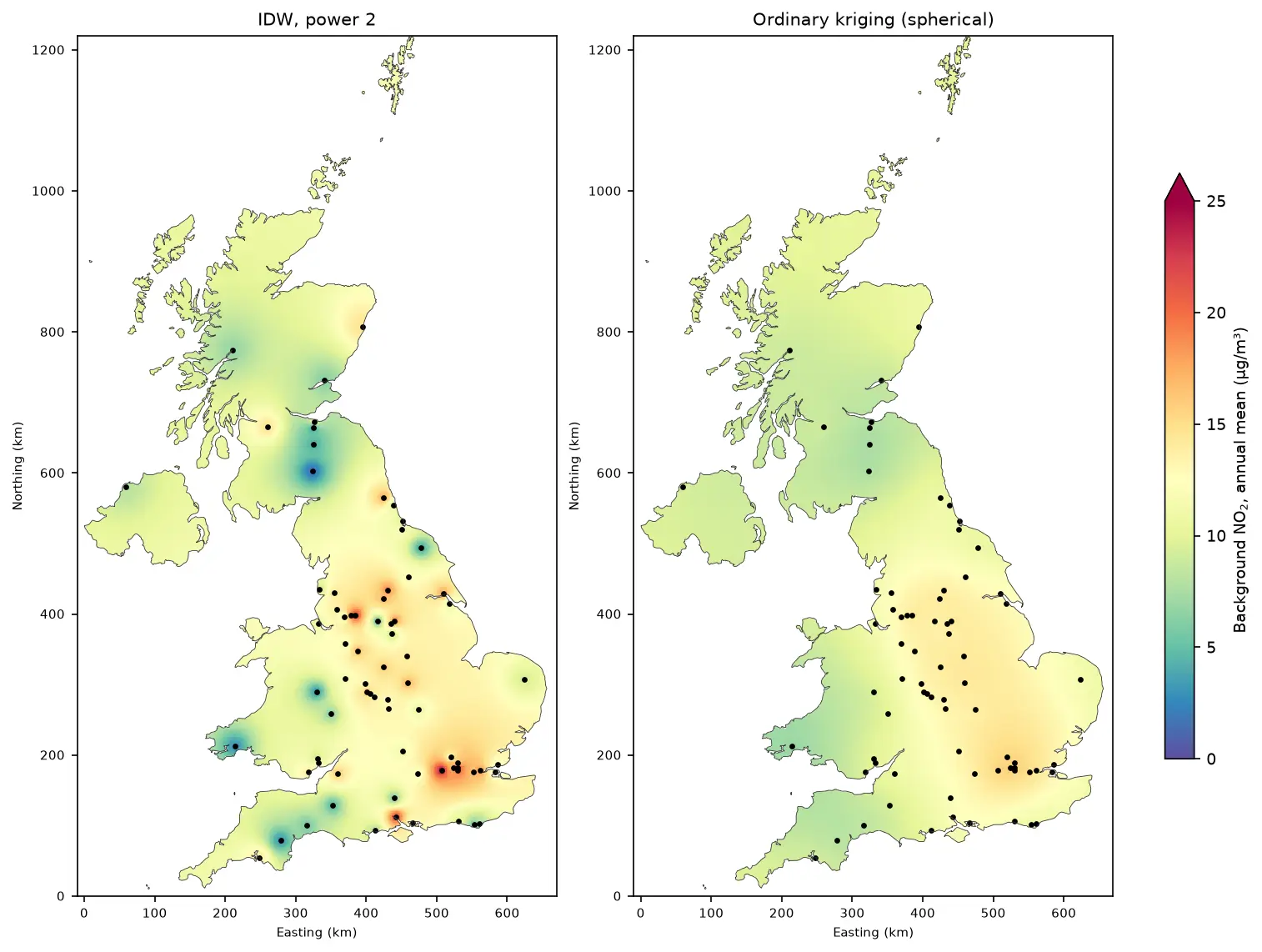
Kriging in Python with PyKrige: IDW vs ordinary kriging of UK NO₂ monitoring data

A practical spatial interpolation tutorial in Python: download real 2025 NO₂ annual means from the UK AURN network, fit spherical, exponential and Gaussian variograms, run ordinary kriging with PyKrige, compare it with inverse distance weighting, score both with leave-one-out cross-validation, map the kriging variance and add Sentinel-5P satellite NO₂ as a covariate.

Intermediate 16 min read

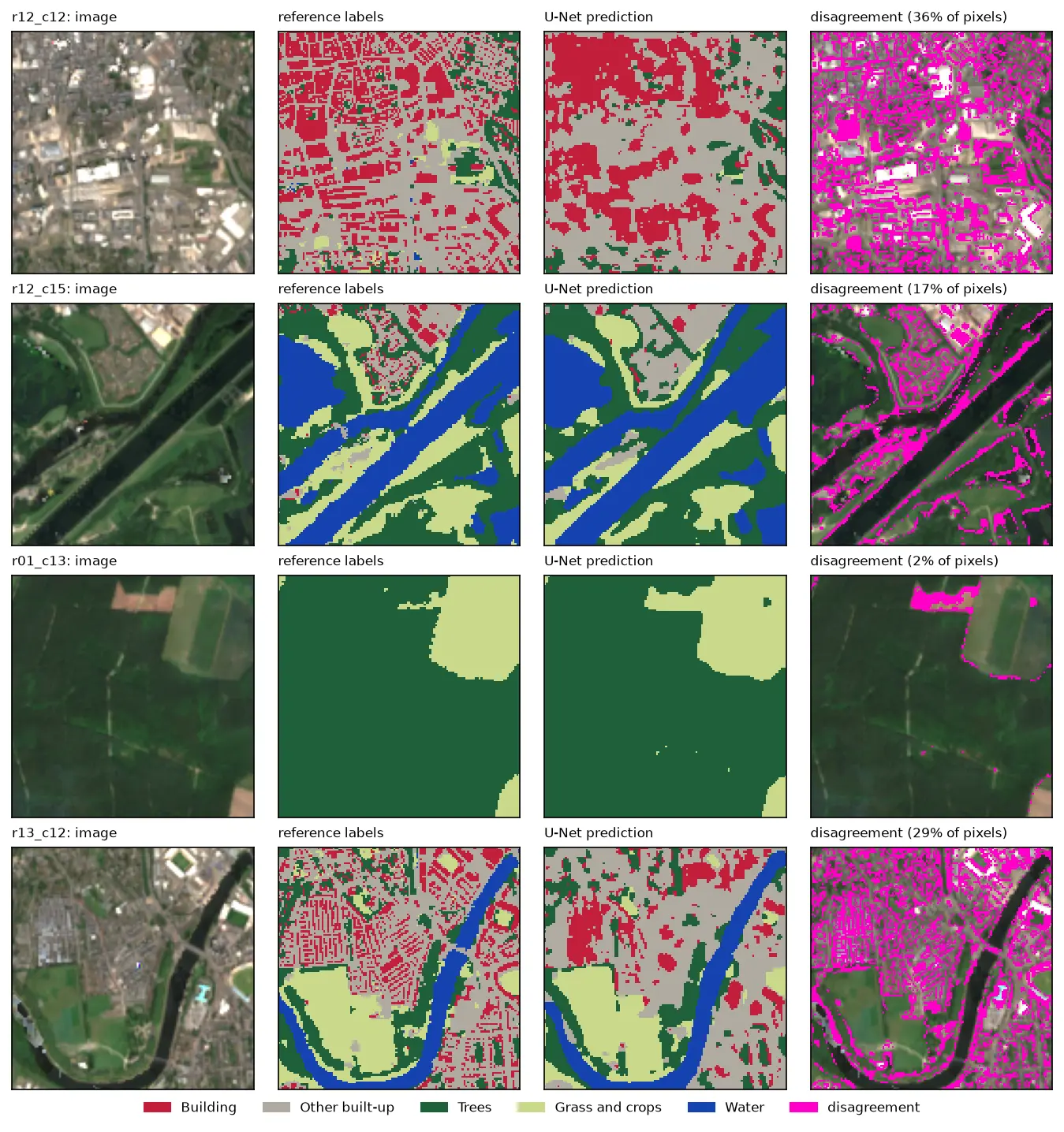
Four rows of Sentinel-2 test chips. Each row shows the image, the reference labels, the U-Net prediction and the disagreement in magenta. The prediction matches rivers, woods and fields closely, but in the city centre it draws buildings as blobs instead of separate roofs.

Tutorial Python Part 2 of 3

U-Net satellite image segmentation in PyTorch: a TorchGeo and Sentinel-2 tutorial on a CPU

Train a U-Net to segment Sentinel-2 imagery into buildings, built-up land, trees, grass and water with PyTorch, segmentation_models_pytorch and TorchGeo's Sentinel-2 pretrained ResNet-18 weights, on a CPU in five minutes. Real loss curves, per-class IoU and F1, a confusion matrix and an honest look at what limits accuracy.

Advanced 12 min read

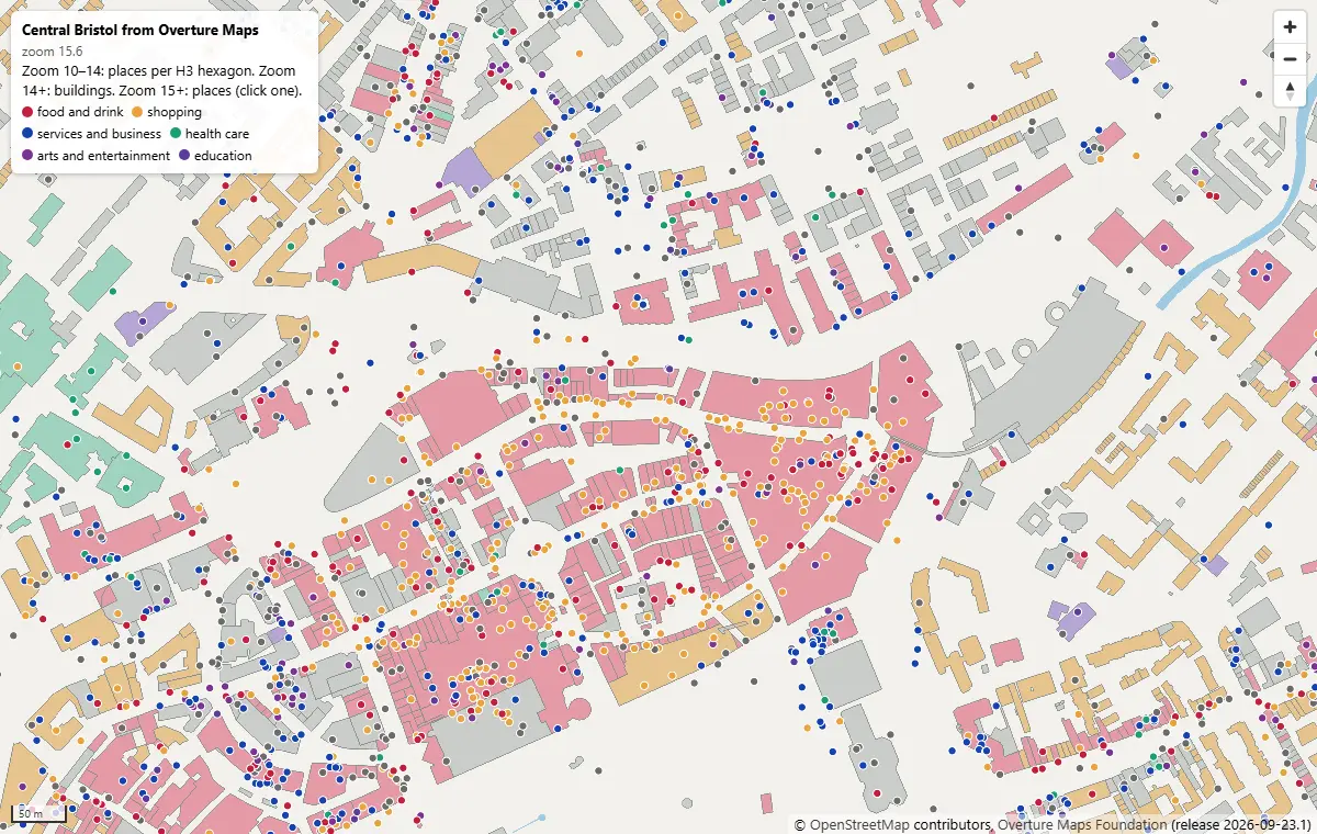
MapLibre GL JS map of central Bristol at zoom 15.6, with Overture building footprints coloured by subtype and places as coloured dots by category, around Broadmead and Cabot Circus

Tutorial Python Part 2 of 2

PMTiles vector tiles in Python and a MapLibre GL JS web map

Turn Overture Maps GeoParquet into PMTiles vector tiles with the GDAL that ships in pyogrio, no Tippecanoe needed, measure the zoom-level and size trade-offs, and serve an interactive MapLibre GL JS map of Bristol from static hosting.

Intermediate 12 min read

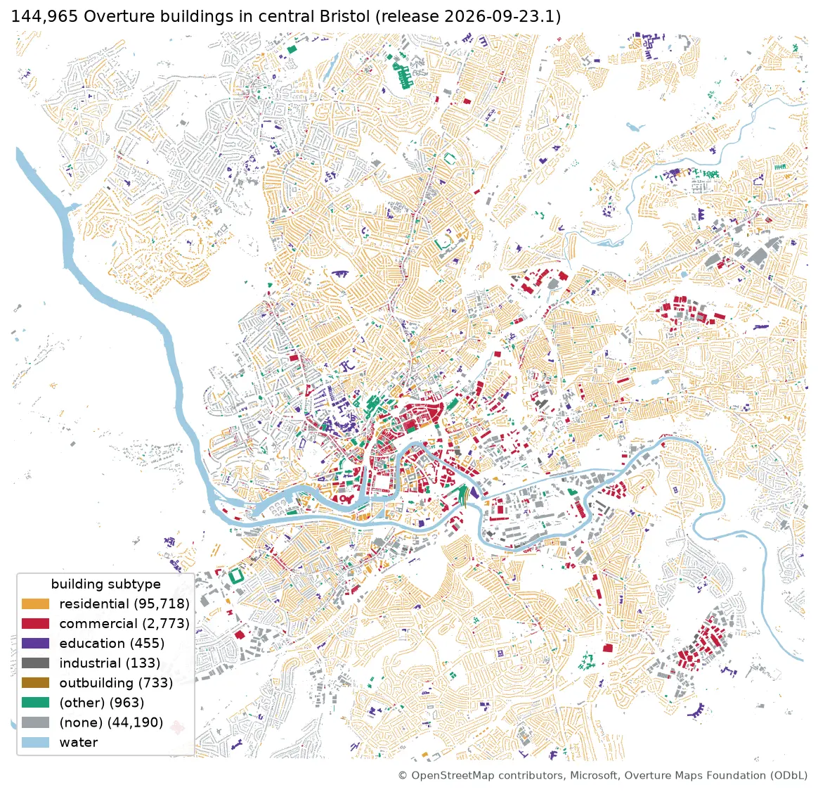
Map of central Bristol with 144,965 Overture building footprints coloured by subtype, most of them residential, and the River Avon in blue

Tutorial Python Part 1 of 2

Query Overture Maps with DuckDB spatial and GeoParquet in Python

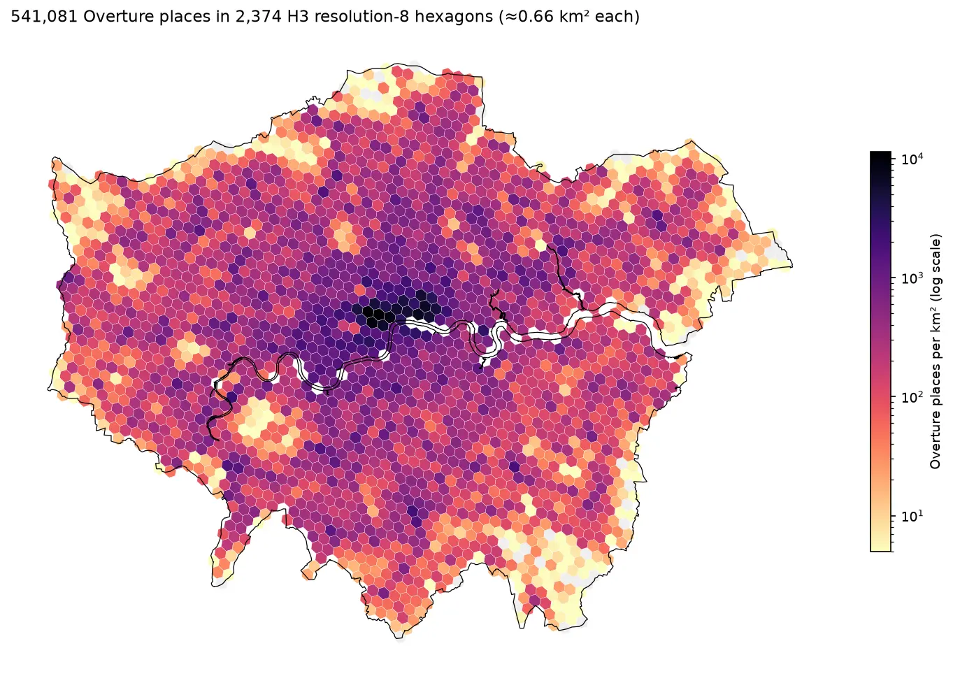
Pull Bristol's 144,965 buildings and 20,727 places straight from the Overture Maps GeoParquet release with DuckDB, run spatial SQL joins and H3 aggregation, load the result into GeoPandas, write GeoParquet 1.1, and time it against Shapefile, GeoPackage and FlatGeobuf.

Intermediate 13 min read

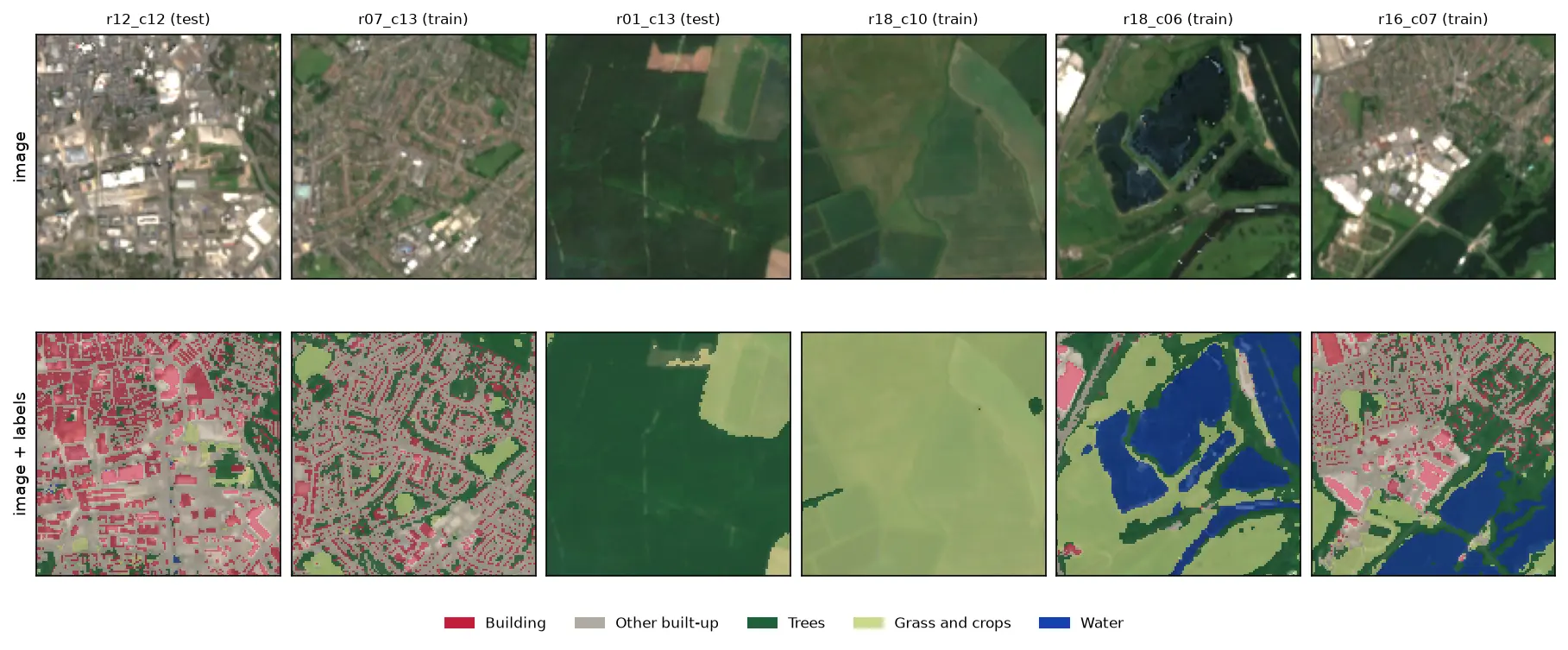
Six 128 by 128 pixel Sentinel-2 image chips of Nottingham, each shown above the same chip with its label mask overlaid: a city centre with red buildings and grey streets, a suburb, a forest, farmland, flooded gravel pits in blue and an industrial estate.

Tutorial Python Part 1 of 3

Training data for deep learning on satellite imagery: Sentinel-2 image chips in Python

Build a labelled deep learning dataset from free data: stream a Sentinel-2 L2A composite from the Planetary Computer, rasterise Overture building footprints over ESA WorldCover, cut georeferenced image chips, split them by spatial block so the test set does not leak, check the class balance and load it all as a TorchGeo dataset.

Intermediate 13 min read

Tutorial Python Part 1 of 2

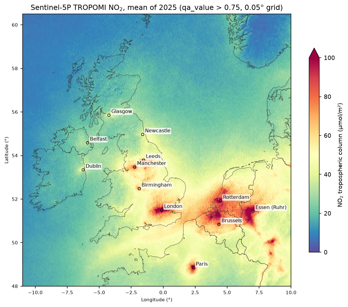
Sentinel-5P NO₂ in Python: mapping air pollution from TROPOMI over the UK and north-west Europe

Map nitrogen dioxide air pollution from Sentinel-5P TROPOMI Level-2 data in Python: stream a full year of orbits from the Planetary Computer, apply the qa_value > 0.75 filter, grid swaths to a regular raster, build monthly and seasonal composites, rank cities and measure the weekend drop, with an honest explanation of what a tropospheric column is.

Intermediate 17 min read

Tutorial Python

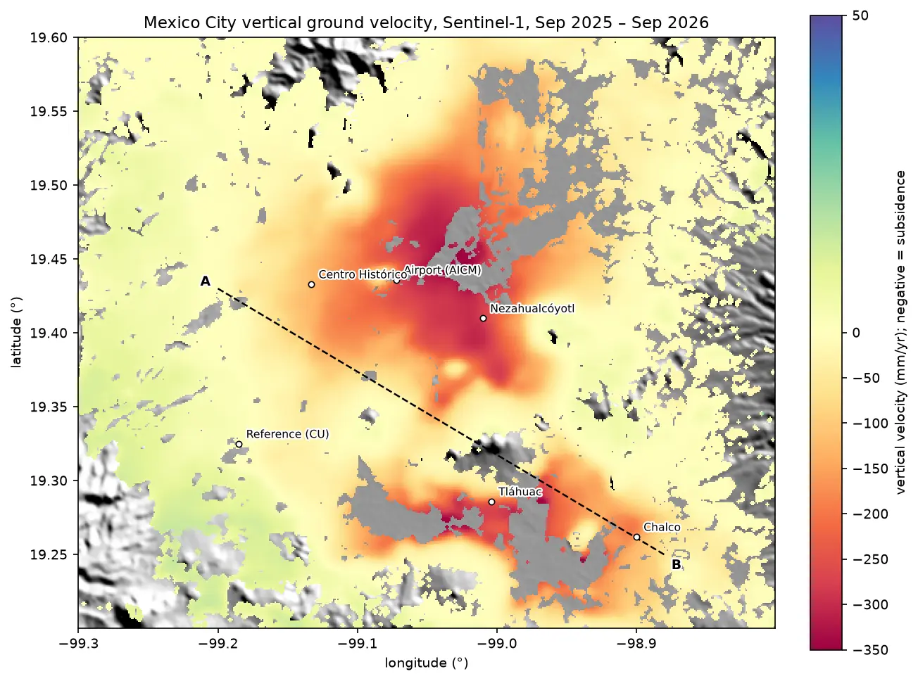
InSAR ground subsidence in Python: one year of Mexico City sinking, from Sentinel-1

Map ground subsidence with Sentinel-1 InSAR in Python: stream 170 real interferograms of Mexico City, convert unwrapped phase to millimetres of line-of-sight motion, mask low coherence, invert a small-baseline network into a time series, and cross-check the velocity with MintPy.

Advanced 17 min read

Tutorial Python

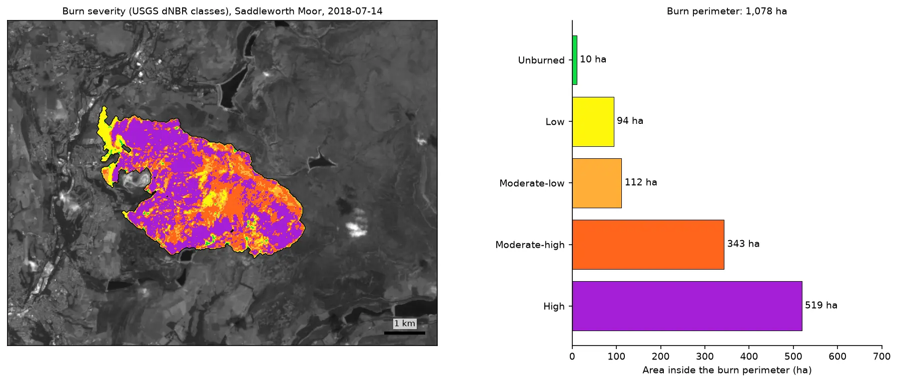
Burn severity mapping with Sentinel-2 and dNBR in Python (Saddleworth Moor 2018)

Map wildfire burn severity in Python with free Sentinel-2 imagery: NBR calculation, cloud and water masking with SCL, dNBR with an offset, USGS severity classes and burned hectares, a burn perimeter, fire progression, RdNBR and an eight-year recovery record for the 2018 Saddleworth Moor fire.

Intermediate 15 min read

Tutorial Python

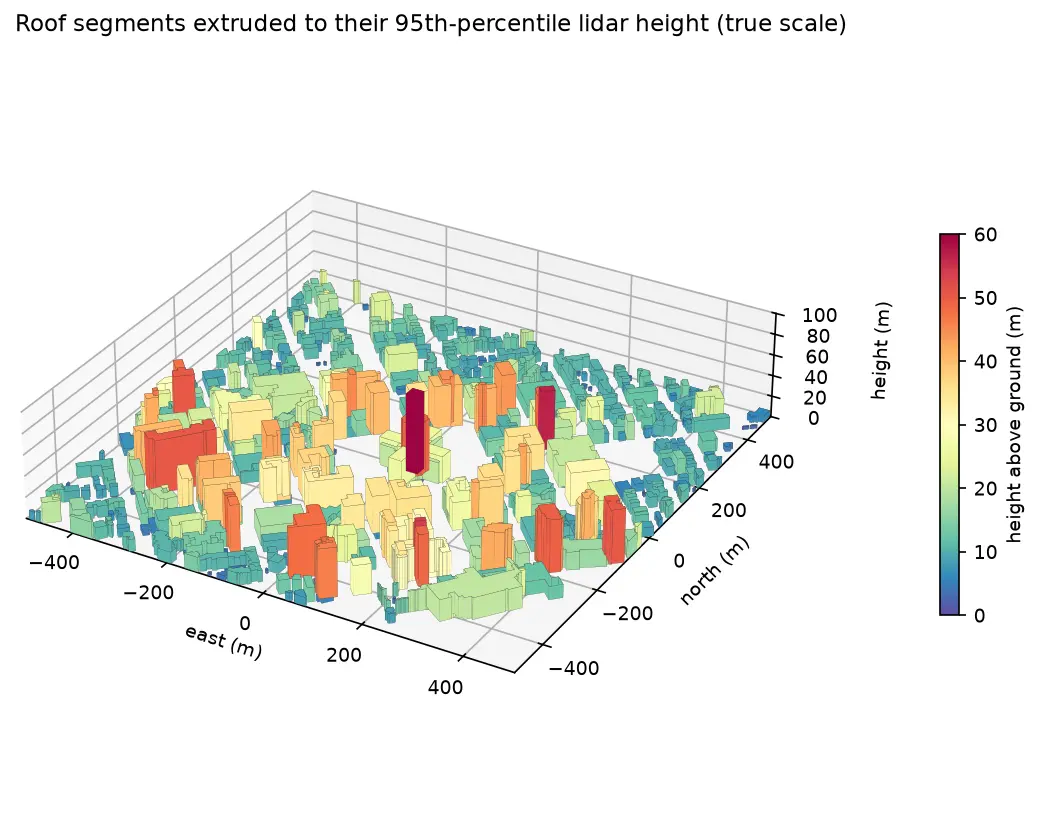
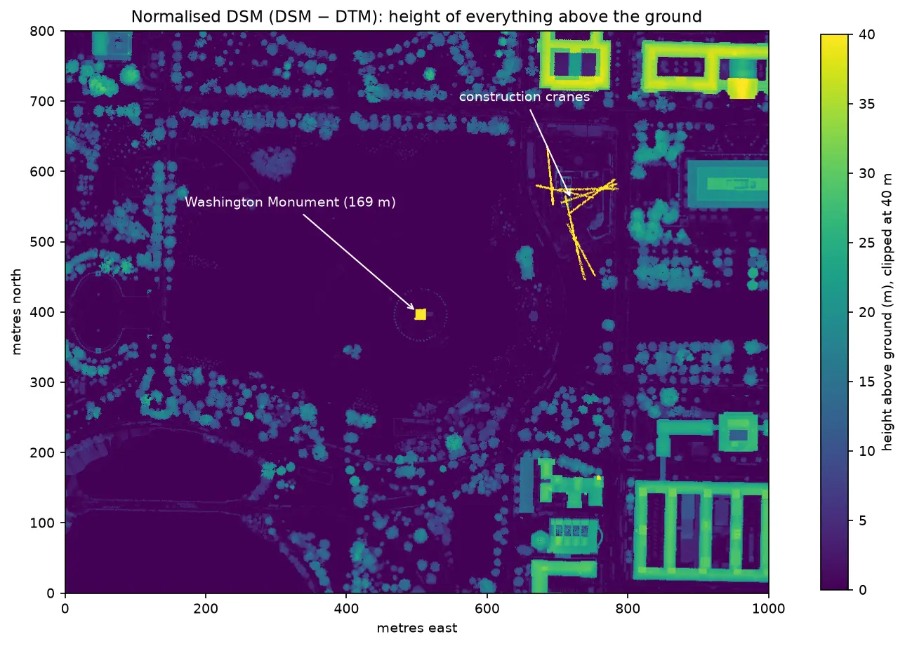
Extract building footprints and heights from LiDAR in Python (USGS 3DEP, downtown Madison)

Turn classified LiDAR into building footprints with heights in Python: stream USGS 3DEP COPC tiles, build a DTM and a building nDSM from ASPRS class 6 points, polygonise and regularise the mask, split roofs at height steps, compute height statistics per building, score the result against OpenStreetMap with IoU, and export a GeoPackage and a 3D view.

Intermediate 15 min read

Tutorial Python

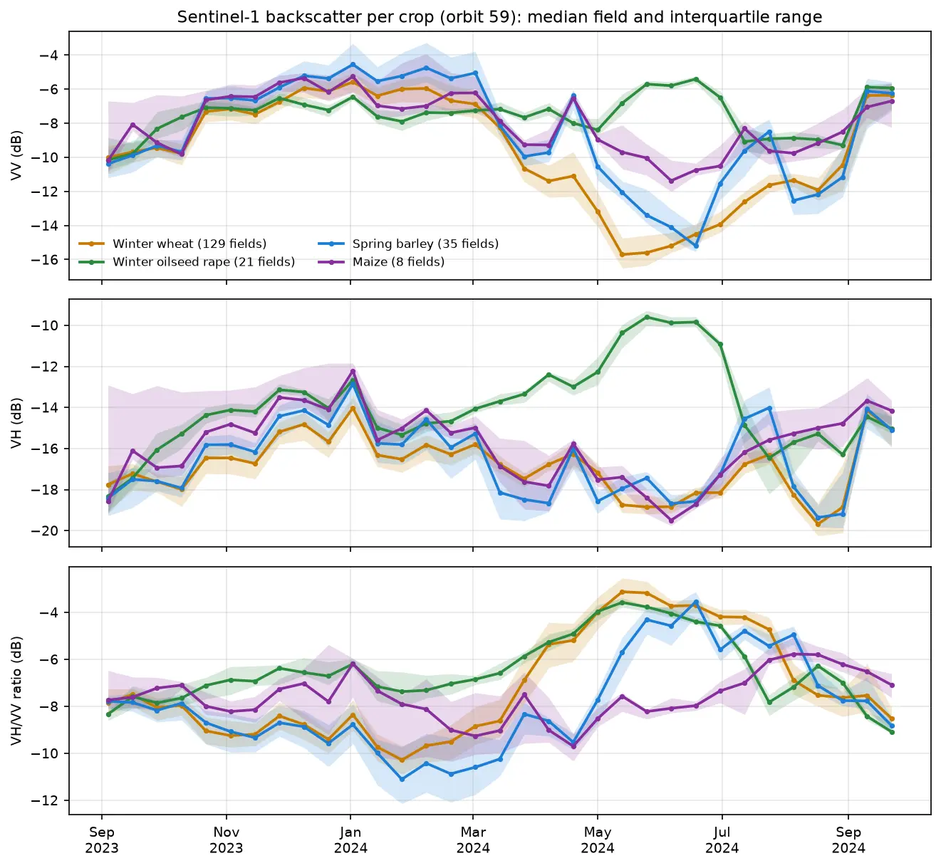
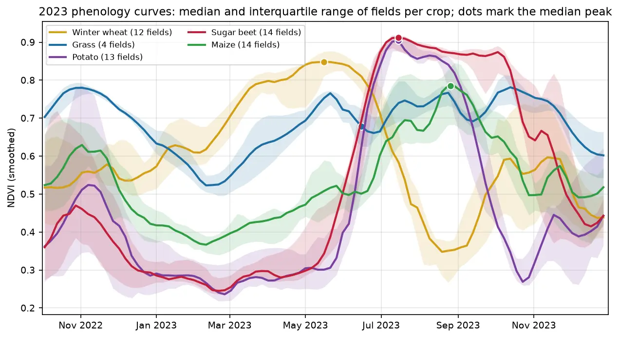
Sentinel-1 crop monitoring in Python: SAR time series for wheat and oilseed rape

Monitor crops through cloud with free Sentinel-1 radar. Build VV, VH and VH/VV ratio time series for 247 fields in Cambridgeshire, beat speckle by field-averaging, read the growth signatures of winter wheat and oilseed rape, and compare with the gaps that cloud leaves in Sentinel-2 NDVI.

Intermediate 16 min read

Tutorial Python

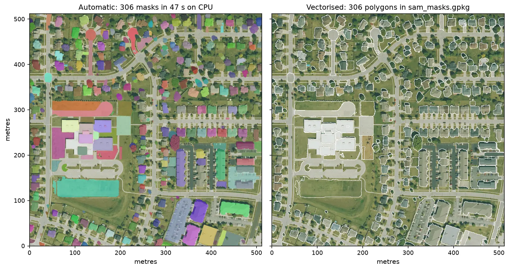
Segment Anything on satellite and aerial imagery in Python: a samgeo tutorial

Run Meta's Segment Anything Model on high-resolution aerial imagery with segment-geospatial (samgeo), on a CPU. Generate masks automatically, vectorise them to a GeoPackage, filter them by area, shape and NDVI to find buildings, and prompt SAM with points and boxes, checked against OpenStreetMap.

Intermediate 14 min read

Tutorial Python

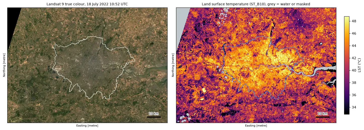
Land surface temperature from Landsat in Python: mapping London's urban heat island

Calculate land surface temperature from Landsat 8 and 9 Collection 2 Level-2 data in Python: ST_B10 scale and offset, QA_PIXEL cloud masking, LST by land cover and NDVI, an urban-rural transect, hotspots with OpenStreetMap and an honest comparison with air temperature, for London in the July 2022 heatwave.

Intermediate 17 min read

Tutorial Python

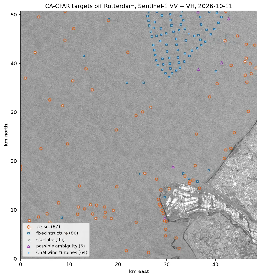
Sentinel-1 ship detection in Python: a CA-CFAR detector off the Port of Rotterdam

Detect ships in free Sentinel-1 SAR imagery with a cell-averaging CFAR detector written in NumPy and SciPy: mask the land, set a threshold from a speckle model, cluster detections into targets, reject wind turbines, sidelobes and ambiguities, compare VV with VH and export the vessels as GeoJSON.

Intermediate 16 min read

Tutorial Python

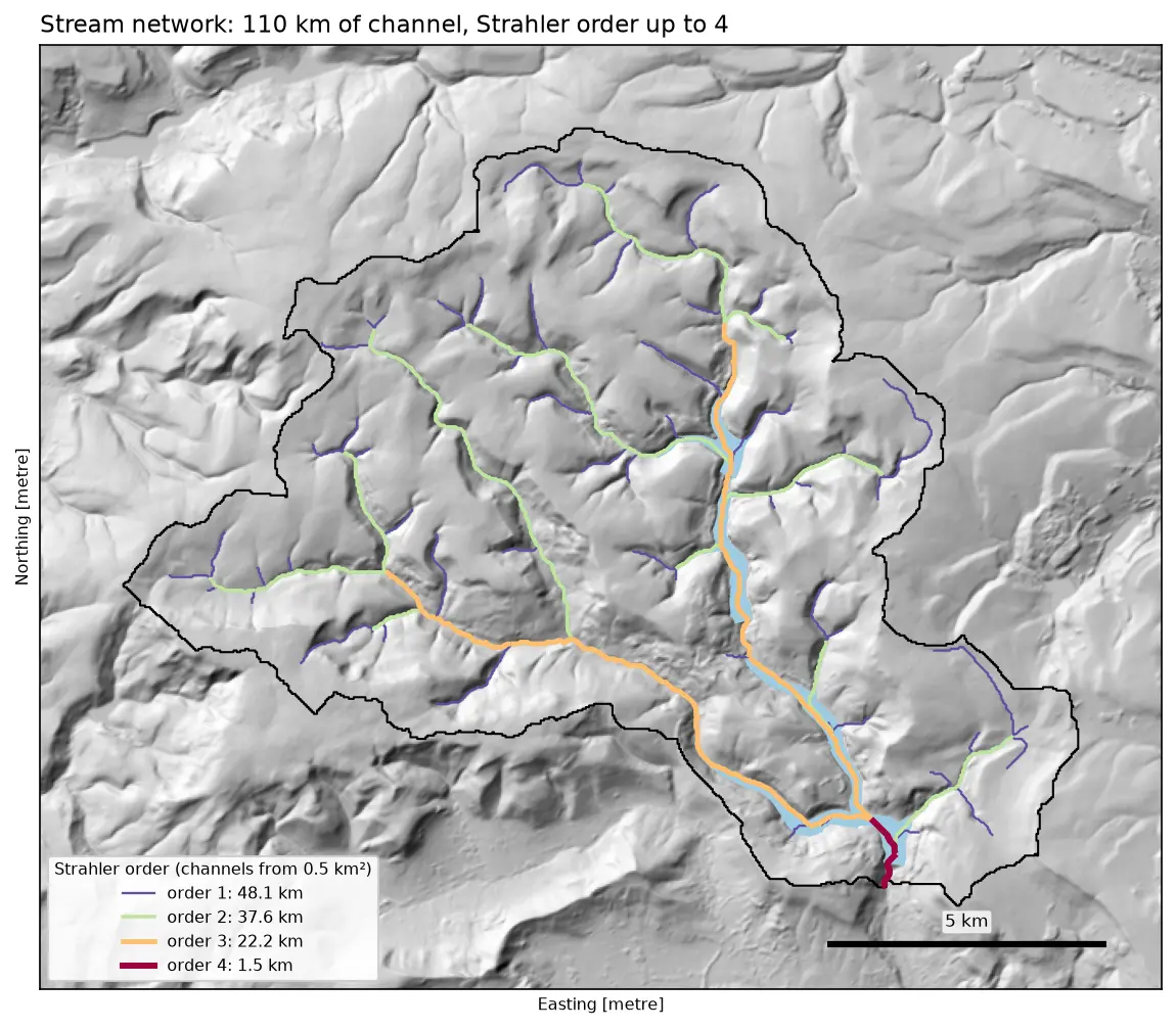
Watershed delineation in Python with pysheds: the River Derwent above Ladybower

Delineate a catchment and its stream network from a free DEM in Python with pysheds: fill pits and depressions, D8 flow direction, flow accumulation, snapping the pour point, catchment polygon and area, Strahler stream order and drainage density, all checked against the official NRFA boundary for the River Derwent at Yorkshire Bridge in the Peak District.

Intermediate 13 min read

Tutorial Python

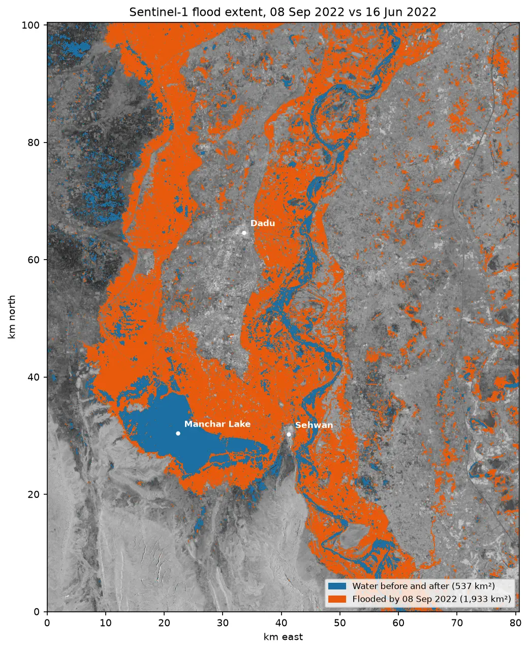
Sentinel-1 SAR flood mapping in Python: the 2022 Pakistan floods

Map the 2022 Sindh floods with free Sentinel-1 radar from the Microsoft Planetary Computer: convert backscatter to decibels, remove speckle with a Lee filter, pick a water threshold with Otsu's method, and measure the flood extent and how it receded over seven months.

Intermediate 10 min read

Tutorial Python Part 1 of 5

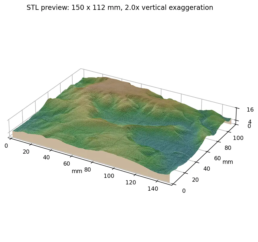
From DEM to 3D-printable STL with Python and NumPy

Stream a Copernicus 30 m DEM of the Edale valley, reproject it to British National Grid, scale it to a 150 mm print and write a watertight binary STL using only NumPy, with checks that prove the mesh is printable.

Intermediate 6 min read

Tutorial Python

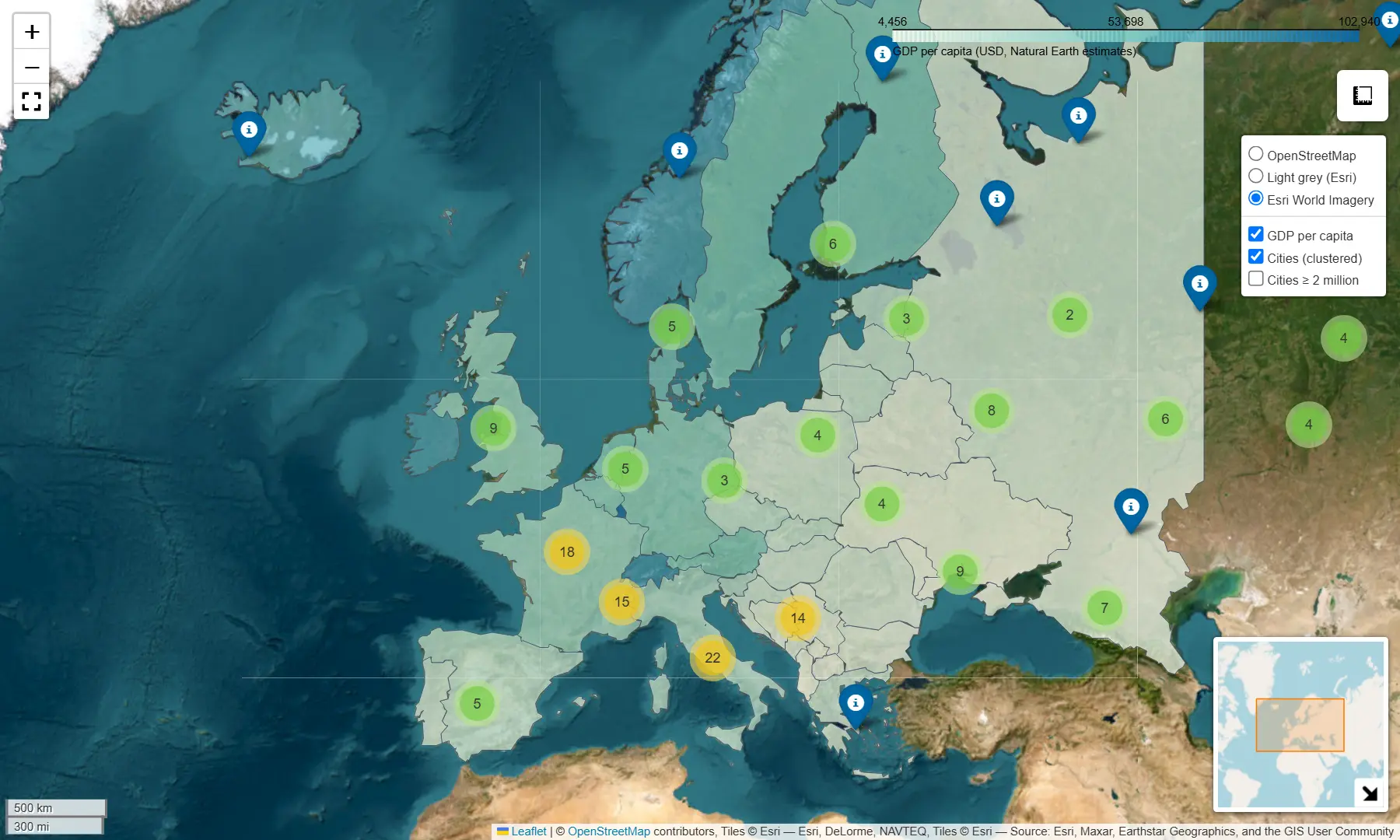
Interactive web maps from Python with Folium and GeoPandas .explore()

Turn GeoDataFrames into shareable Leaflet web maps: a one-line choropleth with .explore(), then a hand-built Folium map with custom styling, tooltips, clustered markers, switchable basemaps and plugins — saved as a single HTML file.

Beginner 5 min read