3D

Terrain models, 3D scenes and printing elevation data.

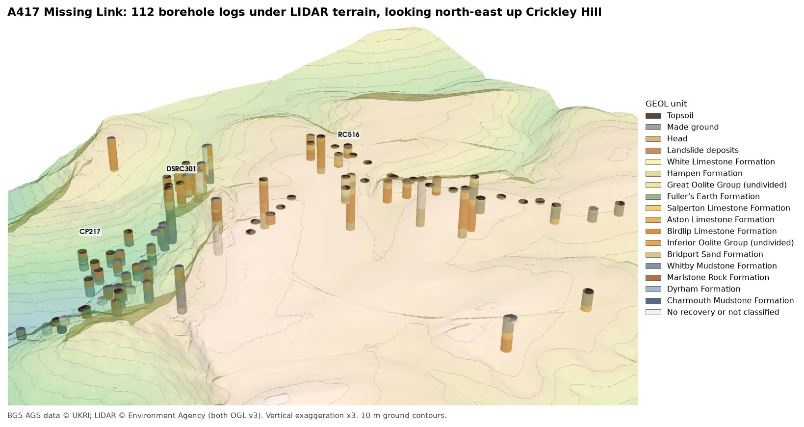
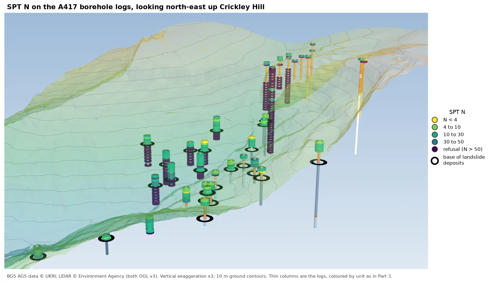
3D view looking north-east up Crickley Hill over semi-transparent LIDAR terrain with 10 m contours. Thin borehole logs coloured by unit carry stacks of coloured discs, one per SPT: yellow and green discs for low N-values near the top of the holes on the escarpment, changing to dark purple refusal discs below black rings that mark the base of the landslide deposits. On the plateau at the top right, the holes turn purple within a few metres of the surface.

Tutorial Python Part 6 of 7

Visualising SPT N-values from AGS4 data in Python

Read the Standard Penetration Tests (ISPT) from a real AGS4 file, separate full tests from refusals, find the stratum each test was made in, and show the N-values four ways: by unit against elevation, across the base of a landslide, as coloured discs on 3D borehole logs over LIDAR terrain, and as a map of the depth to the first refusal.
Intermediate 10 min read

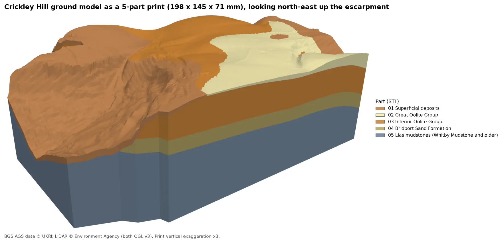
Rendered 3D print of the Crickley Hill ground model, 198 by 145 by 71 mm, looking north-east up the escarpment. Brown superficial deposits cover the western slope, orange Inferior Oolite forms the scarp and plateau, pale yellow Great Oolite caps the south-east, and the side walls show a band of olive Bridport Sand over blue-grey Lias mudstones.

Tutorial Python Part 7 of 7

3D-print a geological ground model: one watertight STL per stratum

Turn the kriged stratum surfaces from Part 5 into a multi-material 3D print of the Cotswold escarpment at Crickley Hill. Cut a window, decide what is too thin to print, build one solid per unit with mesh booleans, prove the parts fit exactly and are watertight, and write five STLs and a colour 3MF for AMS and MMU printers.

Advanced 11 min read

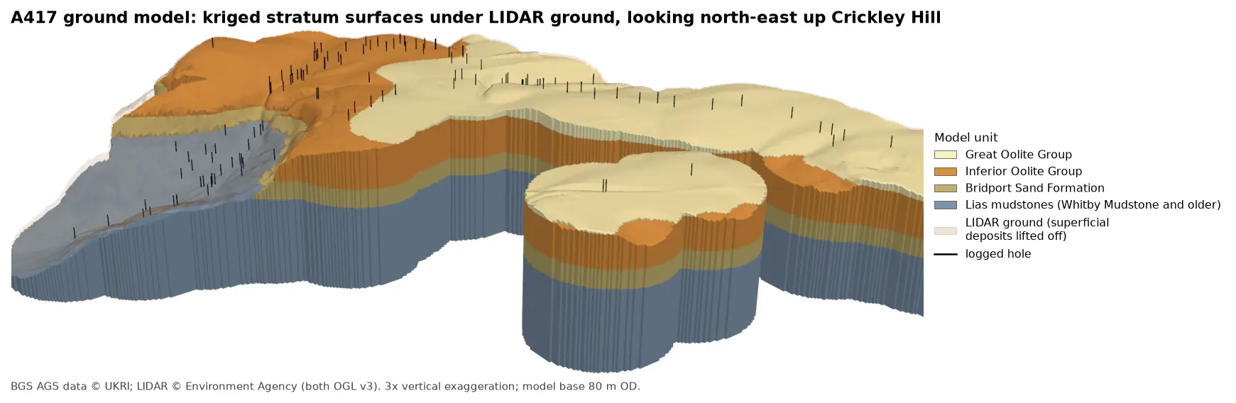
3D block model of the A417 ground model looking north-east up Crickley Hill: blue-grey Lias mudstones form the vale and the lower walls, under a band of olive Bridport Sand, a thick orange band of Inferior Oolite and pale yellow Great Oolite on the plateau. Black vertical lines mark the logged boreholes, and a faint buff skin shows the LIDAR ground lifted off the superficial deposits.

Tutorial Python Part 5 of 7

A 3D ground model from AGS4 boreholes: kriged stratum surfaces in Python

Pick rockhead and the top and base of the key formations from real AGS4 logs, krige them into stratum surfaces under Environment Agency LIDAR ground, and build a 3D ground model of the A417 escarpment in PyVista. Then test it: leave-one-out cross-validation at every borehole, kriging standard deviation maps, a check against every hole that stops short of a surface, and proof that no surface crosses another.

Advanced 15 min read

3D view looking north-east up Crickley Hill: LIDAR terrain shaded from green in the vale to buff on the plateau, with 10 m contours, and 112 borehole logs drawn as vertical cylinders coloured by formation. Blue-grey Lias mudstones fill the holes in the vale, orange Inferior Oolite limestones those on the escarpment, and green Fuller's Earth those on the plateau.

Tutorial Python Part 3 of 7

3D borehole logs from AGS4 data in PyVista and QGIS

Build every borehole log in a real AGS4 file as coloured 3D cylinders at their true elevation under Environment Agency LIDAR terrain with PyVista, then style the same intervals in the QGIS 3D map view. Along the way, test whether neighbouring logs agree, and find a block of ground at the top of Crickley Hill where they don't.

Intermediate 12 min read

Tutorial Python Part 5 of 5

Tiling a large 3D-printed terrain model: jigsaw joints and dowel pins in Python

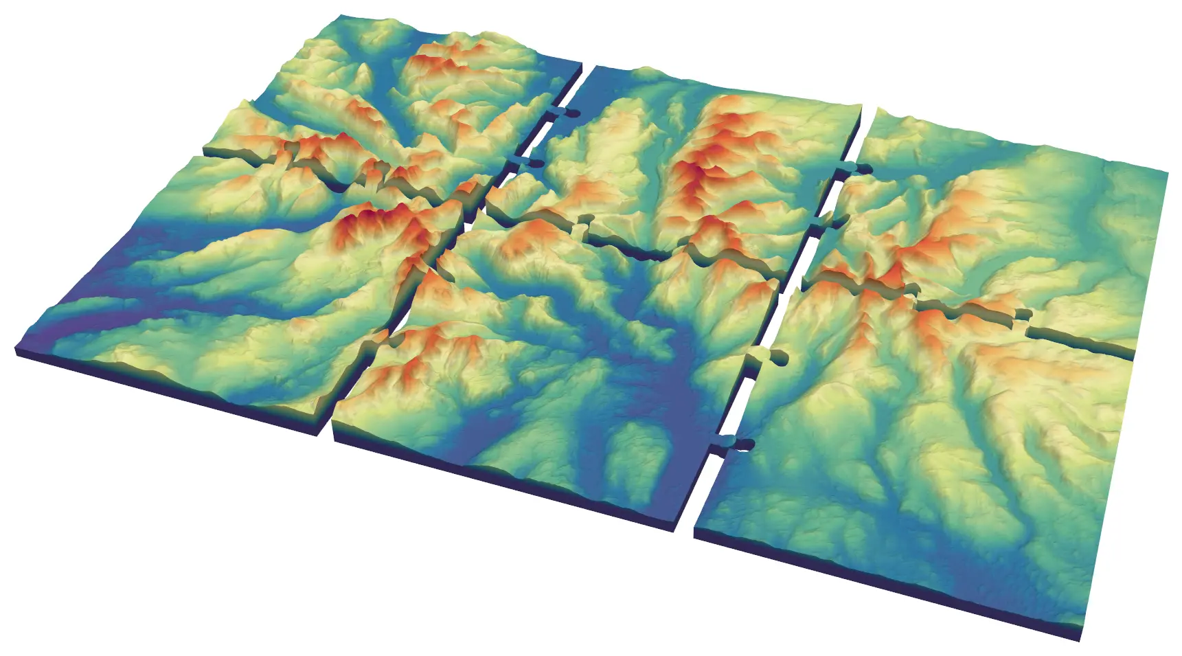
Split a 45 × 30 km model of the central Lake District into six interlocking 150 mm tiles from Copernicus GLO-30, with jigsaw knobs and a 0.2 mm printing clearance or straight edges and filament dowels, and prove every tile is watertight and fits its neighbours.

Advanced 9 min read

Tutorial Python

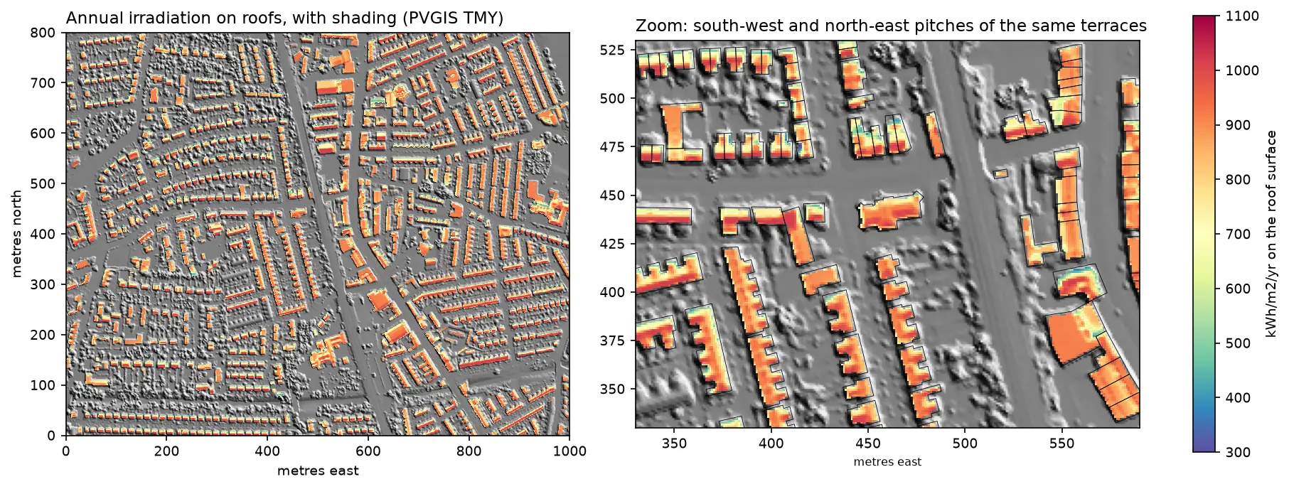
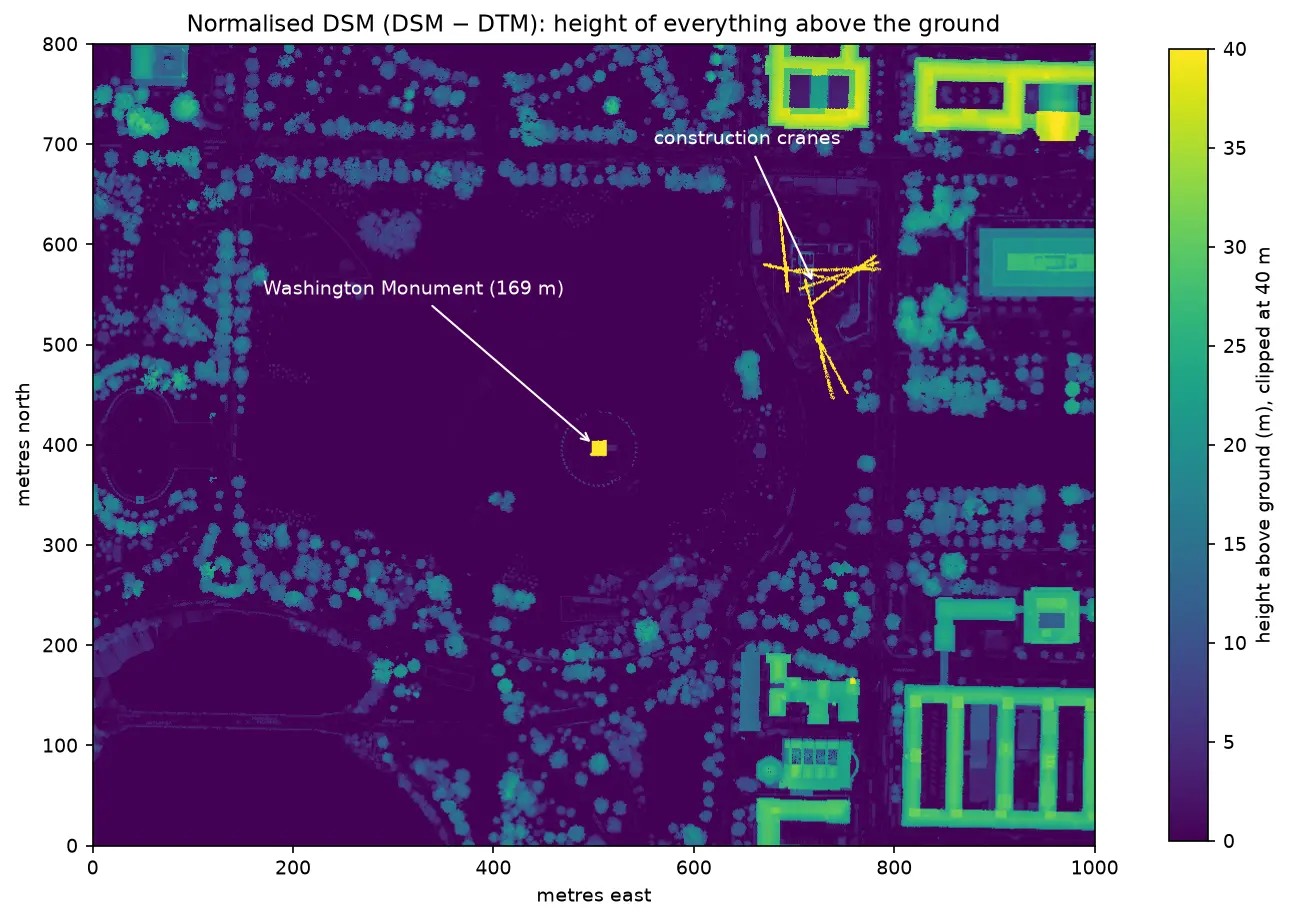
Rooftop solar potential from LiDAR in Python: pvlib, PVGIS and shading for every roof

Estimate rooftop solar potential in Python for 2,148 buildings in Manchester: take a 1 m Environment Agency LiDAR DSM and Overture Maps footprints, compute roof slope and aspect, trace horizon angles for shading from neighbours and trees, build a sun map from a PVGIS typical year with pvlib, check it against pvlib's Perez model and PVGIS, then estimate kWp and kWh per year per roof and rank the best roofs.

Advanced 14 min read

Tutorial Python

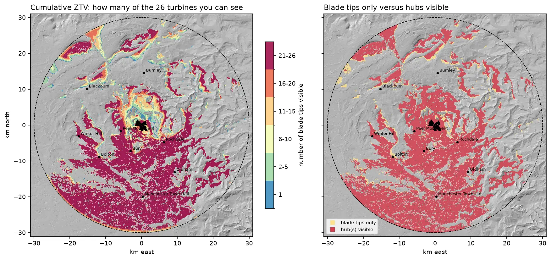
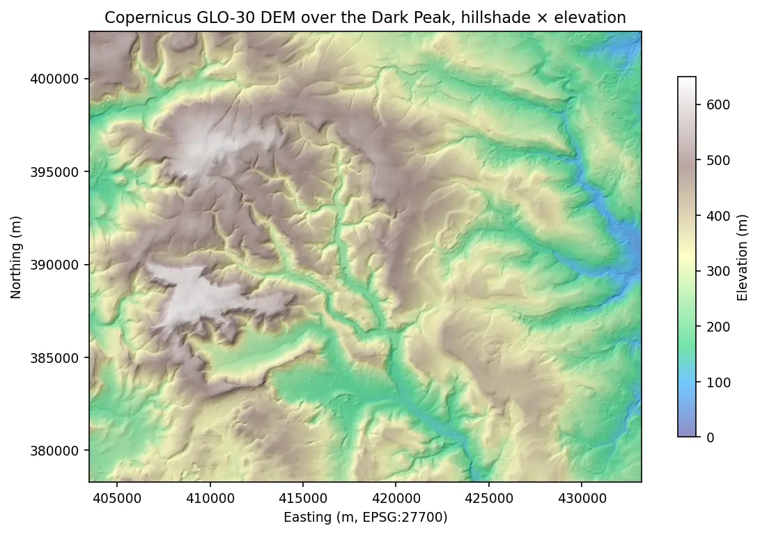
Viewshed analysis in Python: line of sight and a wind farm ZTV with GDAL and numpy

Run a viewshed analysis in Python on a real DEM: compute what one wind turbine can see with gdal.ViewshedGenerate, rebuild the same line-of-sight algorithm in numpy, correct for earth curvature and refraction, build a cumulative zone of theoretical visibility (ZTV) from 26 turbines, draw line-of-sight profiles, and measure how much trees and buildings in a LiDAR DSM shrink a bare-earth viewshed.

Intermediate 16 min read

Tutorial Python

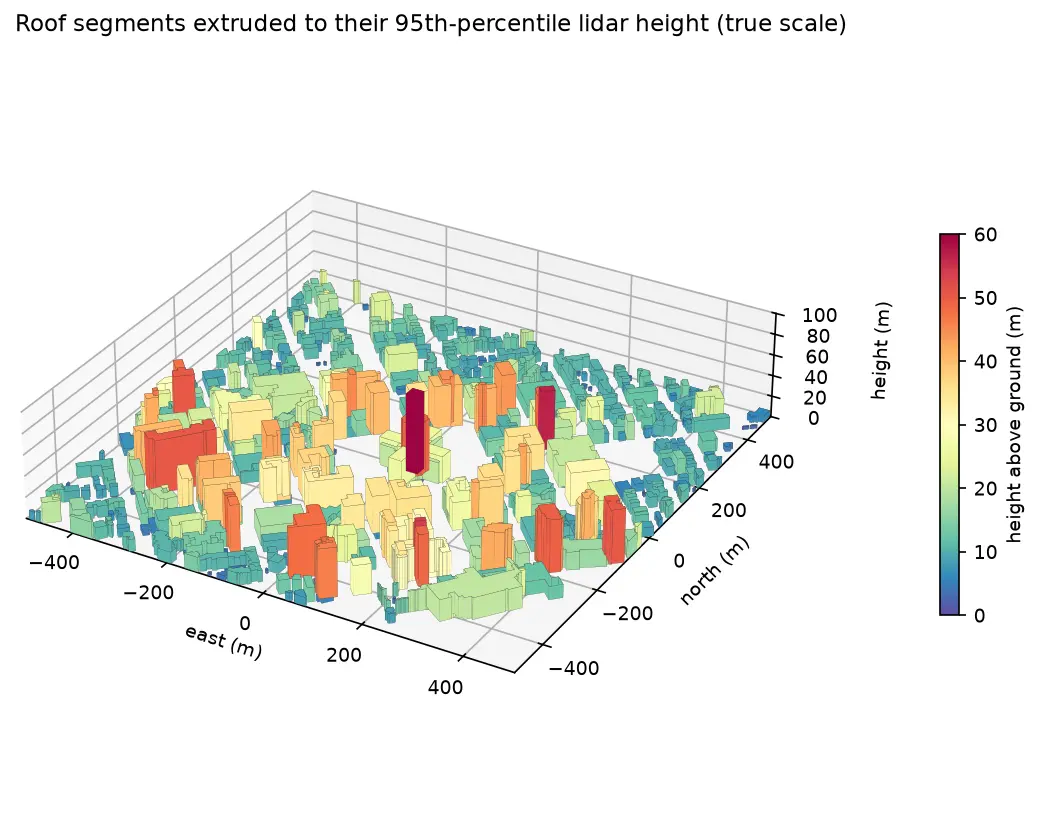
Extract building footprints and heights from LiDAR in Python (USGS 3DEP, downtown Madison)

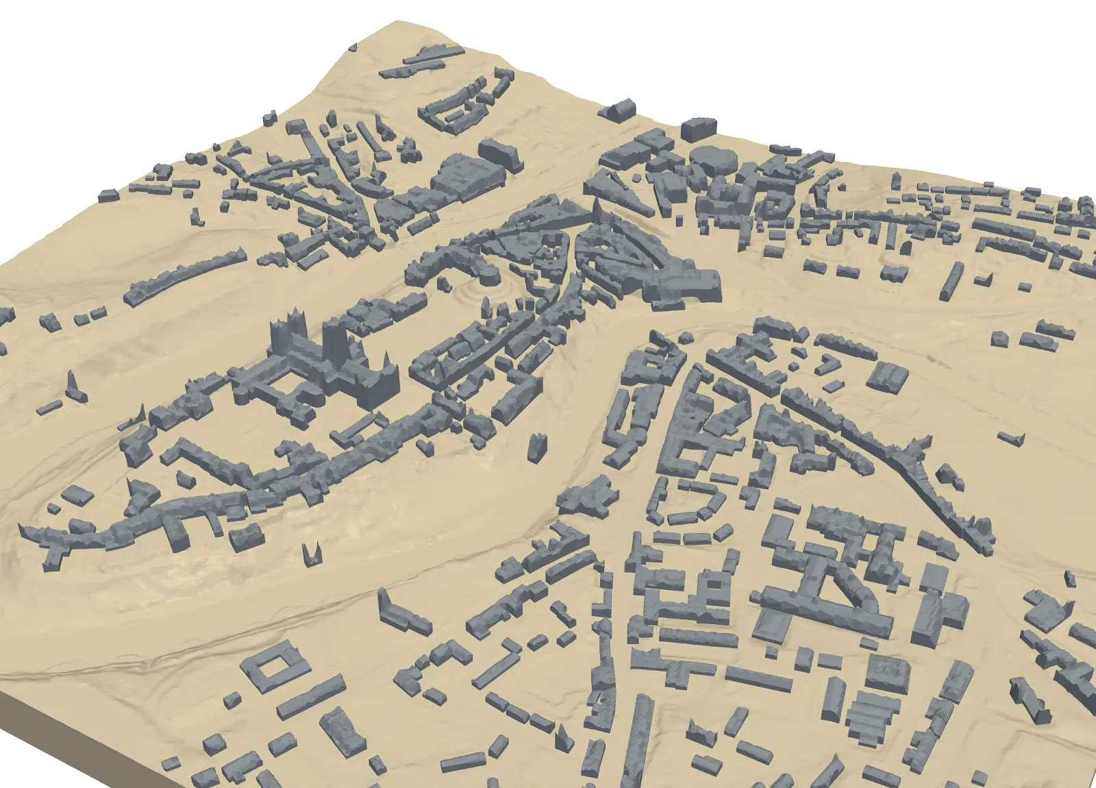
Turn classified LiDAR into building footprints with heights in Python: stream USGS 3DEP COPC tiles, build a DTM and a building nDSM from ASPRS class 6 points, polygonise and regularise the mask, split roofs at height steps, compute height statistics per building, score the result against OpenStreetMap with IoU, and export a GeoPackage and a 3D view.

Intermediate 15 min read

Tutorial Python Part 1 of 5

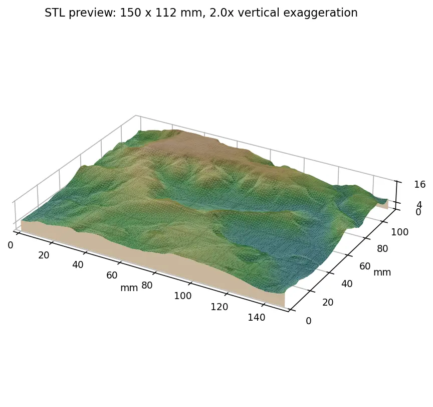
From DEM to 3D-printable STL with Python and NumPy

Stream a Copernicus 30 m DEM of the Edale valley, reproject it to British National Grid, scale it to a 150 mm print and write a watertight binary STL using only NumPy, with checks that prove the mesh is printable.

Intermediate 6 min read

Article ArcGIS Pro

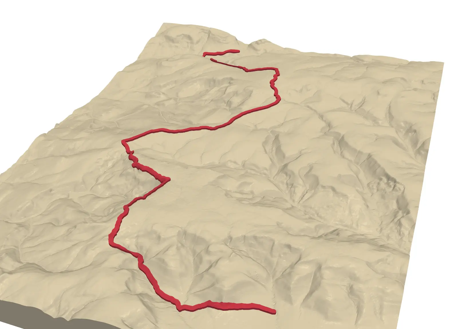
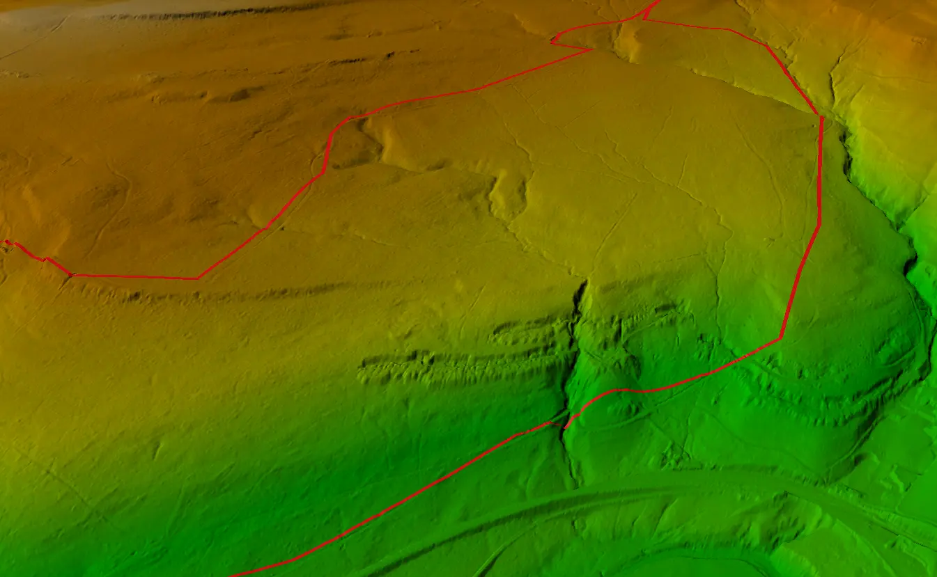
Visualising a Cycle Track in 3D

Turning a GPX track of the Wharncliffe Woods cycle route into a 3D scene and elevation profile in ArcGIS Pro.

Beginner 1 min read