#GeoPackage

4 posts

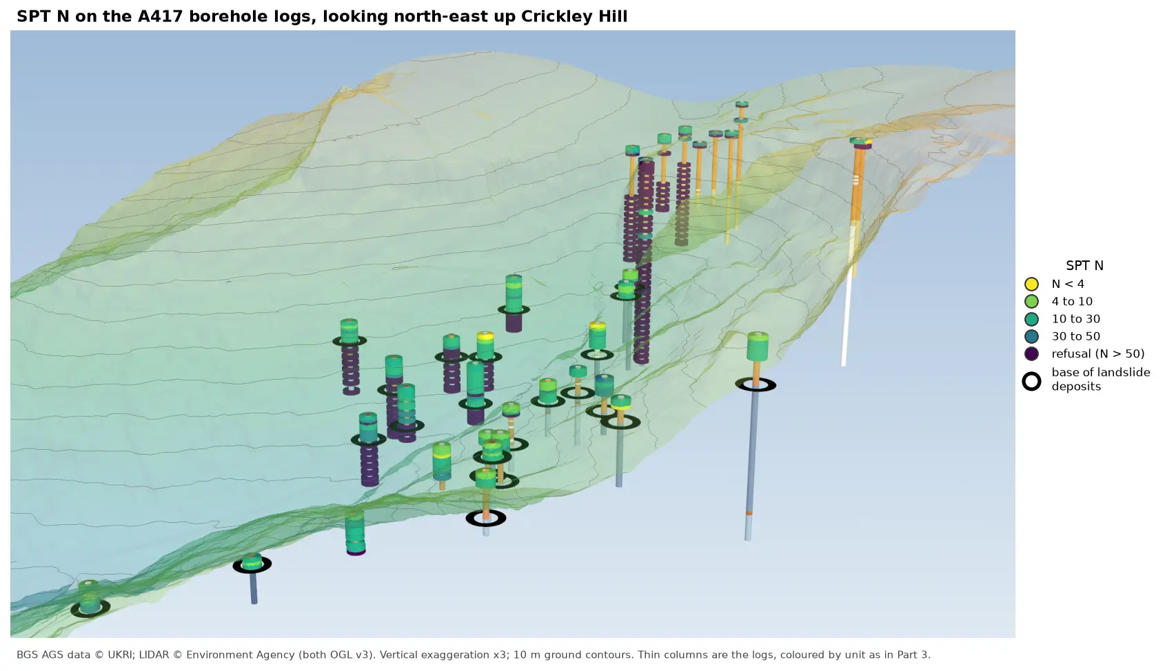
3D view looking north-east up Crickley Hill over semi-transparent LIDAR terrain with 10 m contours. Thin borehole logs coloured by unit carry stacks of coloured discs, one per SPT: yellow and green discs for low N-values near the top of the holes on the escarpment, changing to dark purple refusal discs below black rings that mark the base of the landslide deposits. On the plateau at the top right, the holes turn purple within a few metres of the surface.

Tutorial Python Part 6 of 7

Visualising SPT N-values from AGS4 data in Python

Read the Standard Penetration Tests (ISPT) from a real AGS4 file, separate full tests from refusals, find the stratum each test was made in, and show the N-values four ways: by unit against elevation, across the base of a landslide, as coloured discs on 3D borehole logs over LIDAR terrain, and as a map of the depth to the first refusal.
Intermediate 10 min read

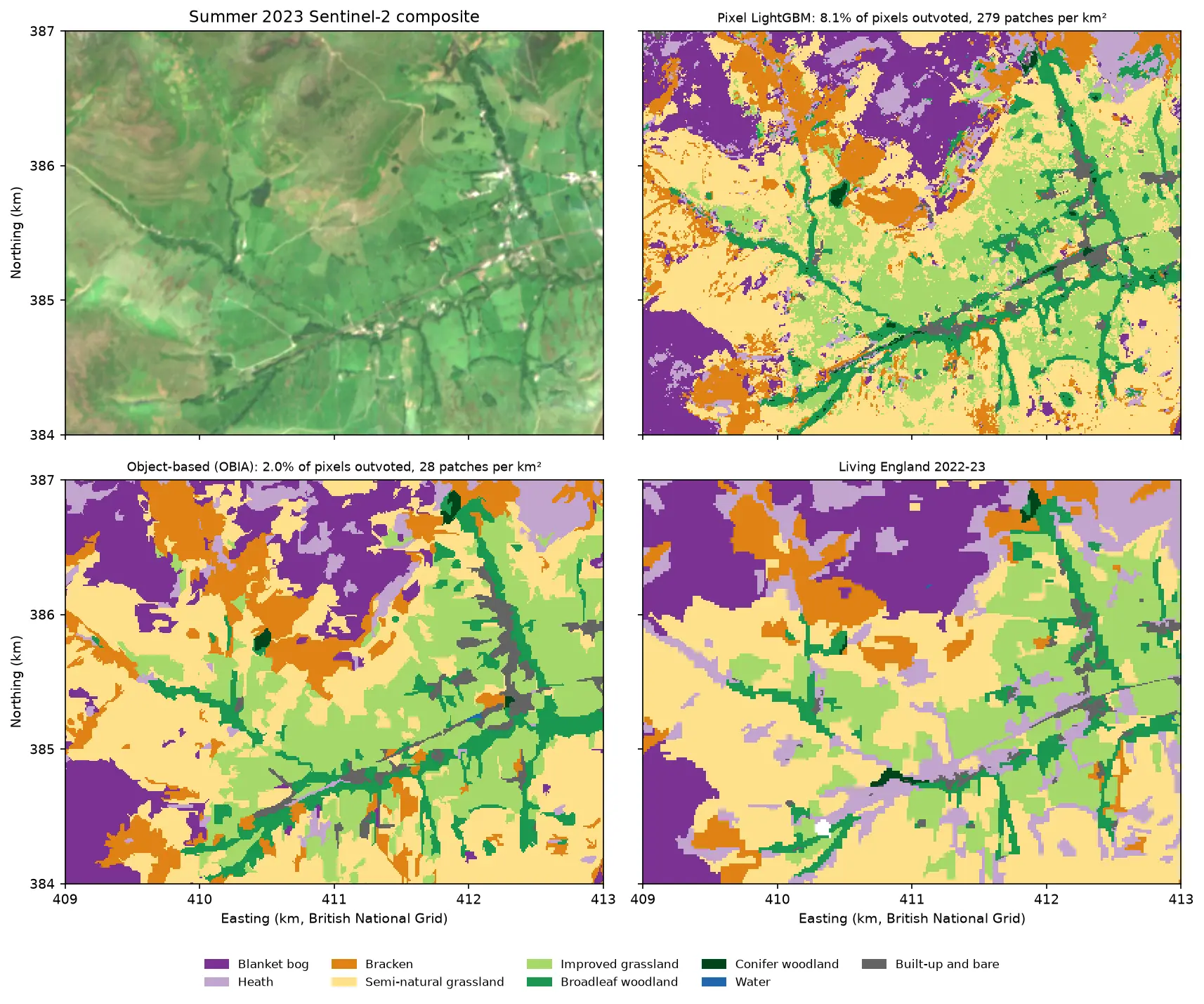
Four panels of the same 4 by 3 km area of the Edale valley and the southern edge of Kinder Scout. Top left: a true colour Sentinel-2 image of green fields and brown moorland. Top right: a pixel-based habitat map speckled with isolated pixels of other classes. Bottom left: the object-based map, with the same habitats in clean patches that follow field boundaries. Bottom right: the Living England reference map.

Tutorial Python Part 3 of 5

Object-based image analysis in Python: OBIA habitat classification with Sentinel-2

Segment 2023 Sentinel-2 seasonal composites of the Peak District into image objects with scikit-image SLIC and Felzenszwalb, tune the segment size against Living England boundaries, compute per-object statistics, shape and GLCM texture with NumPy, classify the objects with LightGBM and compare OBIA with a pixel-based classifier on accuracy, salt-and-pepper noise and patch counts. Then export the habitat objects as GeoPackage polygons.

Advanced 21 min read

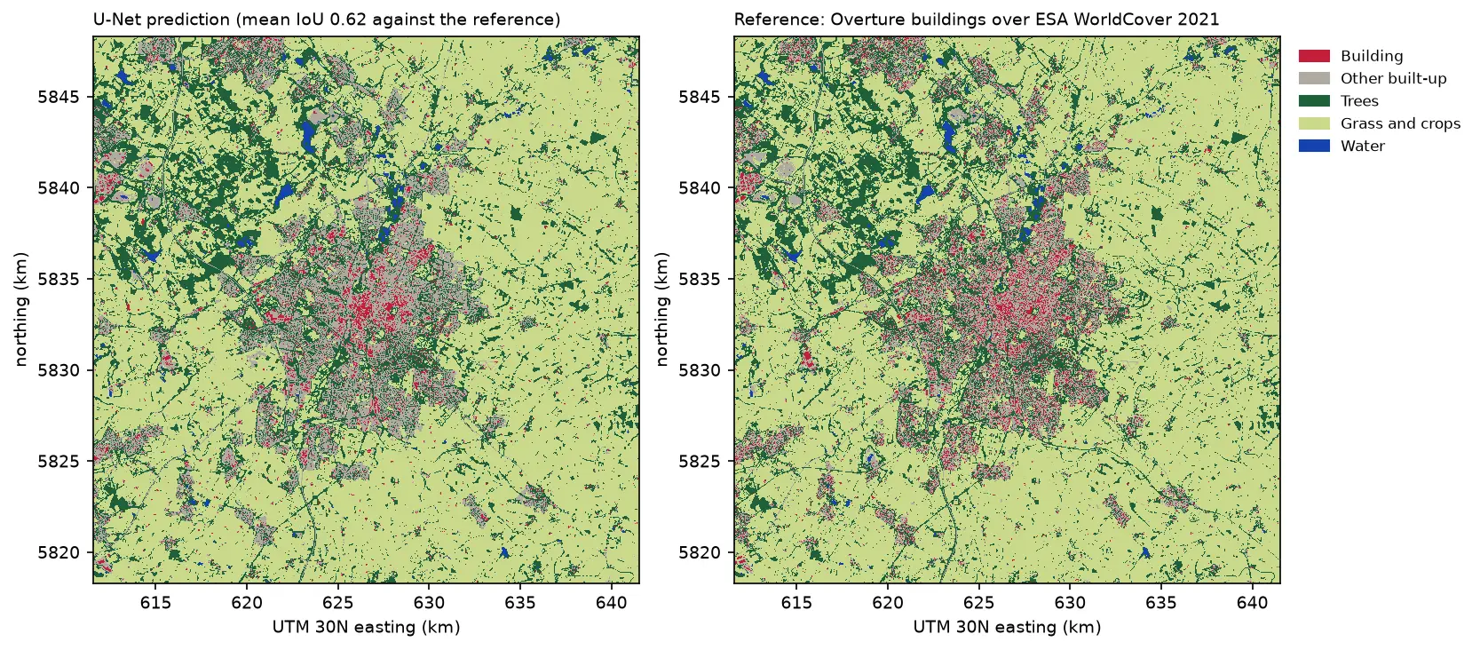
Two land cover maps of a 30 km square around Leicester side by side: the U-Net prediction on the left and the reference labels on the right. Both show the city in grey and red in the centre, surrounded by farmland in pale green, woods in dark green and reservoirs in blue. The prediction's city is smoother, with fewer separate red buildings.

Tutorial Python Part 3 of 3

Deep learning inference on large rasters: sliding-window prediction, COGs and polygons in Python

Run a trained PyTorch U-Net over a whole Sentinel-2 scene of a city it has never seen: tiled sliding-window inference on a large GeoTIFF with overlapping, blended windows, a georeferenced Cloud Optimised GeoTIFF of classes and confidence, raster-to-vector polygons with rasterio.features.shapes in a GeoPackage, and an honest check against reference labels.

Advanced 13 min read

Tutorial Python

Extract building footprints and heights from LiDAR in Python (USGS 3DEP, downtown Madison)

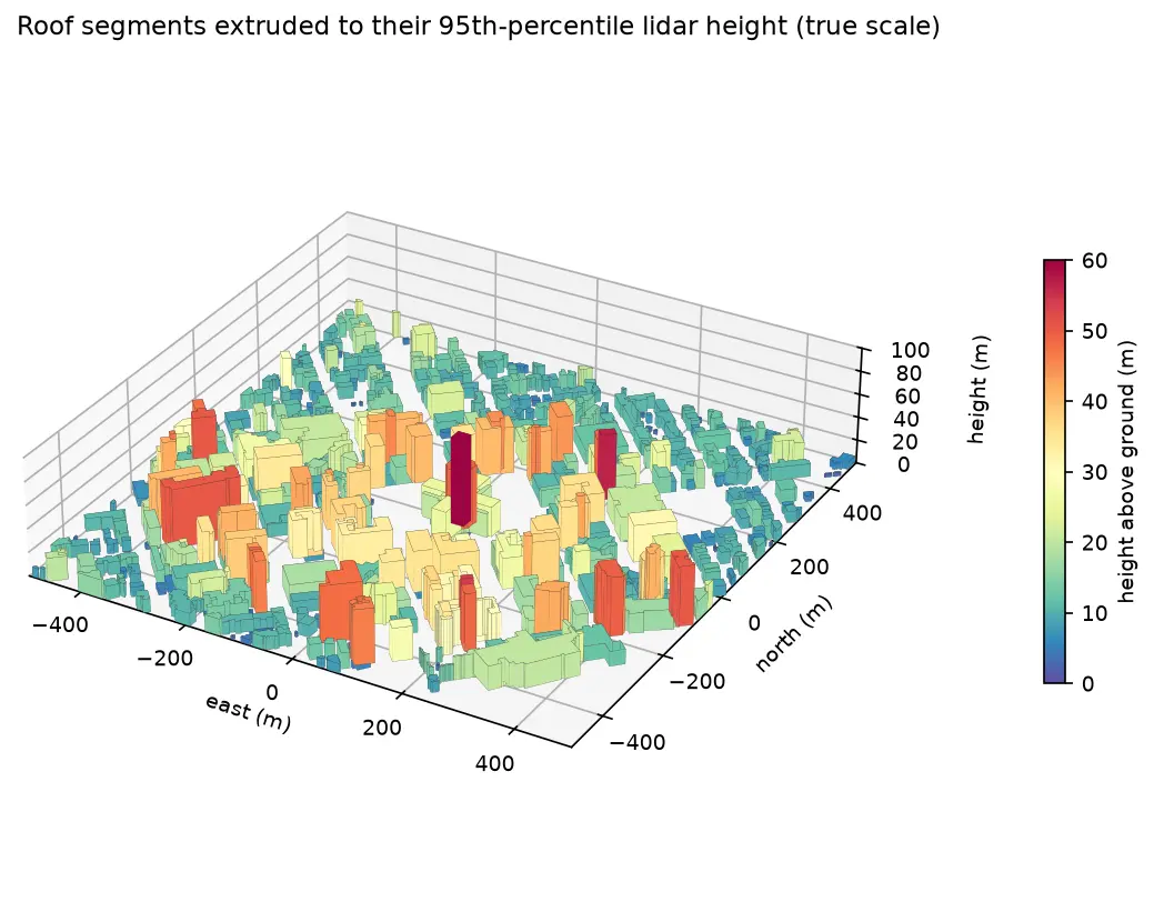
Turn classified LiDAR into building footprints with heights in Python: stream USGS 3DEP COPC tiles, build a DTM and a building nDSM from ASPRS class 6 points, polygonise and regularise the mask, split roofs at height steps, compute height statistics per building, score the result against OpenStreetMap with IoU, and export a GeoPackage and a 3D view.

Intermediate 15 min read