#Matplotlib

3 posts

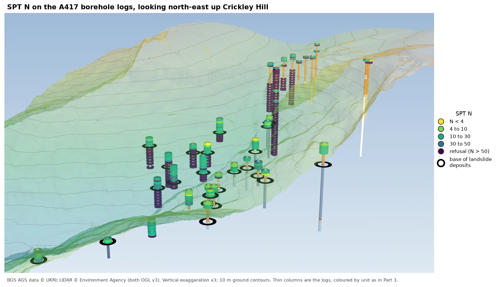
3D view looking north-east up Crickley Hill over semi-transparent LIDAR terrain with 10 m contours. Thin borehole logs coloured by unit carry stacks of coloured discs, one per SPT: yellow and green discs for low N-values near the top of the holes on the escarpment, changing to dark purple refusal discs below black rings that mark the base of the landslide deposits. On the plateau at the top right, the holes turn purple within a few metres of the surface.

Tutorial Python Part 6 of 7

Visualising SPT N-values from AGS4 data in Python

Read the Standard Penetration Tests (ISPT) from a real AGS4 file, separate full tests from refusals, find the stratum each test was made in, and show the N-values four ways: by unit against elevation, across the base of a landslide, as coloured discs on 3D borehole logs over LIDAR terrain, and as a map of the depth to the first refusal.
Intermediate 10 min read

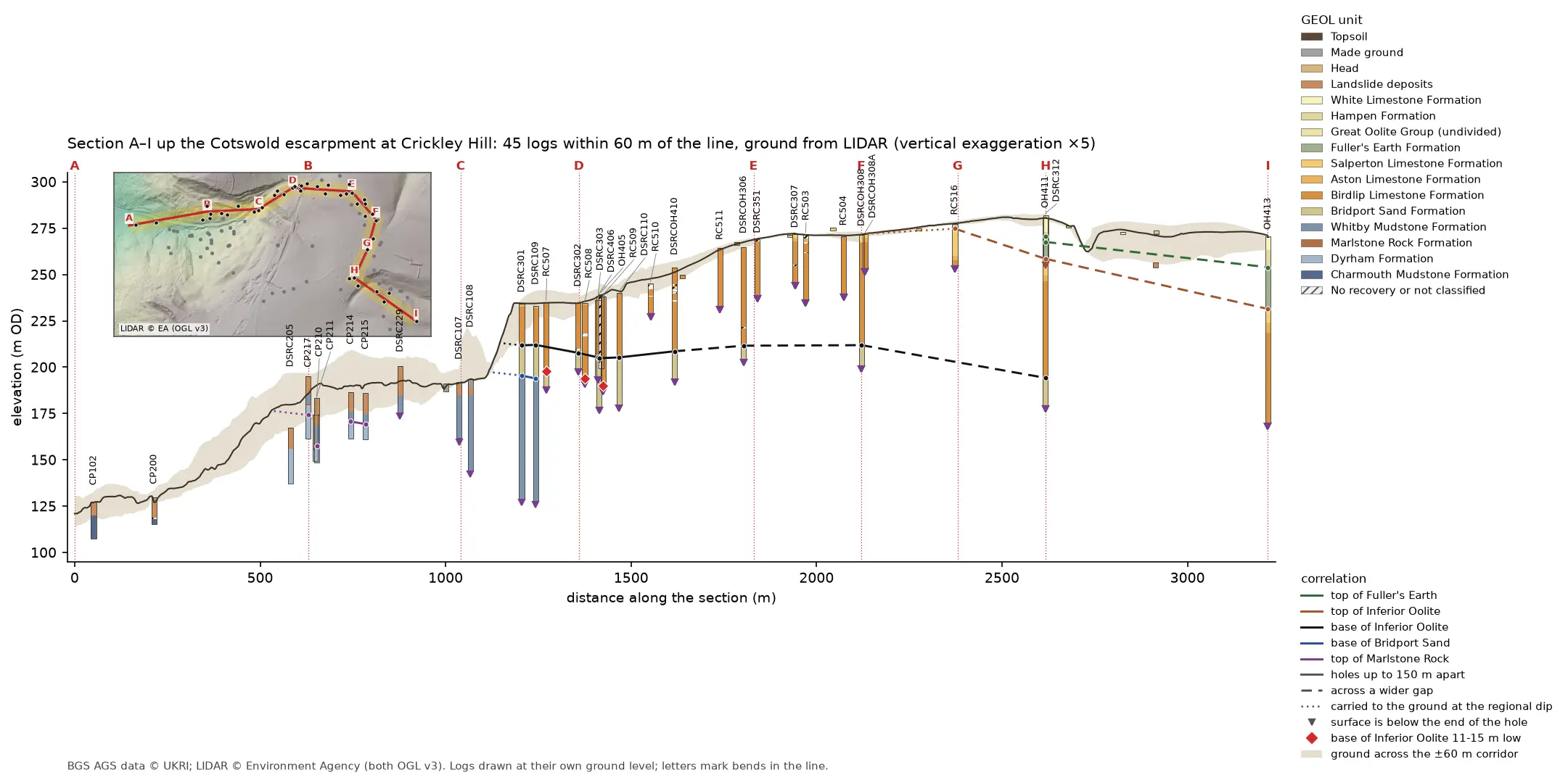
Geological cross-section 3.2 km long from the vale at A, up the Cotswold escarpment at Crickley Hill, to the plateau at I. A dark LIDAR ground line climbs from 121 to 281 m OD over a buff band showing the ground across the corridor. Forty-five strip logs hang below it, coloured by formation: blue-grey Lias mudstone in the vale, orange Inferior Oolite limestone on the escarpment and green Fuller's Earth on the plateau. Coloured lines join the contacts between holes, and red diamonds mark three holes where the base of the limestone is 11 to 15 m low. A map inset at top left shows the bent section line and its corridor on a LIDAR hillshade.

Tutorial Python Part 4 of 7

A geological cross-section from AGS4 boreholes and LIDAR in Python and QGIS

Draw a 3.2 km geological cross-section up the Cotswold escarpment from real AGS4 borehole logs, with the ground profile from Environment Agency LIDAR. Project every hole in a corridor onto the line, pick and correlate the contacts, and measure how much of each correlation line rests on a log and how much is inferred. Then draw the same section with the QGIS elevation profile.

Intermediate 15 min read

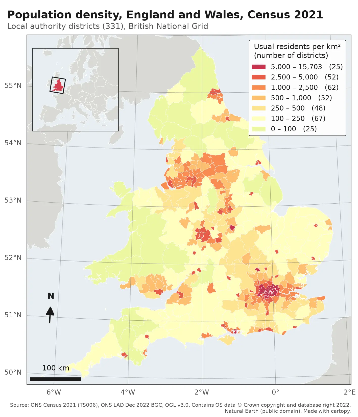
Choropleth map of population density in the 331 local authority districts of England and Wales from Census 2021, in seven classes from pale yellow (under 100 residents per km²) to deep red (over 5,000). London, Birmingham, Manchester, Liverpool, Leeds, Newcastle and the south coast cities stand out in red; Wales, Cumbria, Northumberland and Lincolnshire are pale. The map has a classified legend, a 100 km scale bar, a north arrow, latitude and longitude labels and an inset locator map of Europe.

Tutorial Python

Make a map in Python with matplotlib and cartopy: projections, classified choropleths, scale bars, north arrows and inset maps

A cartopy tutorial for publication-quality maps in Python: choose a projection, draw a classified choropleth of Census 2021 population density with a proper legend, add a scale bar, a true-north arrow, an inset locator map and gridlines, style it for light and dark backgrounds, export at 300 dpi to PNG, PDF and SVG, and shade the Copernicus DEM for Greater Manchester.

Beginner 14 min read