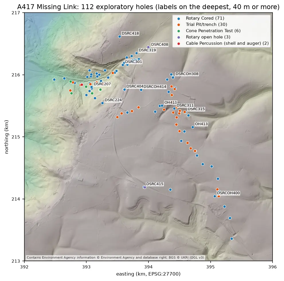
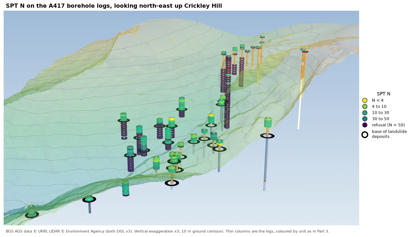
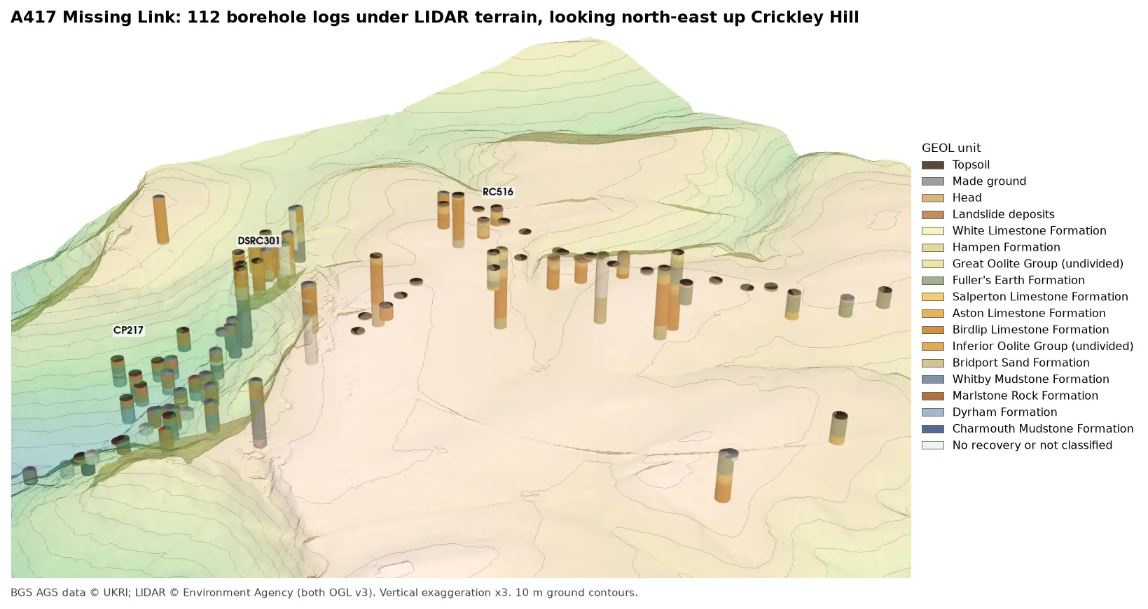
A geological cross-section from AGS4 boreholes and LIDAR in Python and QGIS
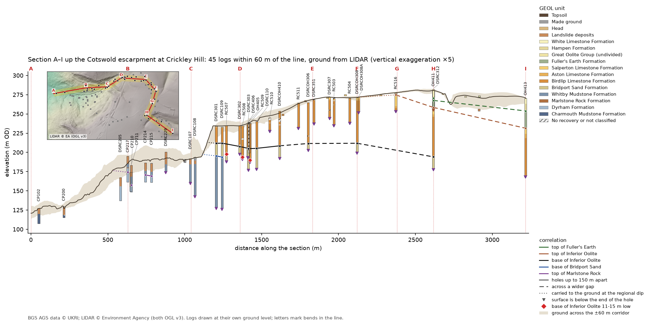
Draw a 3.2 km geological cross-section up the Cotswold escarpment from real AGS4 borehole logs, with the ground profile from Environment Agency LIDAR. Project every hole in a corridor onto the line, pick and correlate the contacts, and measure how much of each correlation line rests on a log and how much is inferred. Then draw the same section with the QGIS elevation profile.
- Level
- Intermediate
- Tested with
- Python 3.12
- Source code
- Download scripts
Key takeaways
- A section line that follows the holes, with a corridor 60 m either side, puts 45 logs on one 3.2 km section. Each hole is projected to the nearest point on the line, and its distance off the line is kept as evidence.
- LIDAR gives a ground profile every 2 m. The A417 collar levels agree with it to a median of 0.09 m, but on the escarpment the ground 54 m off the line can be 15 m lower than on it, so each log is drawn at its own ground level.
- Contacts are picked from the logs by formation order, and neighbouring contacts are joined only if they agree within 3 m or an apparent dip of 5°. Where they disagree, the section says so rather than drawing a line.
- Measuring how much of each correlation line lies within 50 m of a logged contact shows which surfaces rest on logs (the base of the Inferior Oolite, 47%, with all 9 neighbouring pairs agreeing) and which are mostly inferred (the top of the Fuller's Earth, 17%).
- The QGIS elevation profile draws the same section from the same GeoPackage, and its ground profile matches the Python one to a median of 0.05 m.
Before you start
- Part 1 of this series, or at least its helper module a417_ags.py
- Python 3.10+ with python-ags4, GeoPandas, shapely, rasterio, SciPy, requests and matplotlib
- QGIS 3.34 or later for the elevation profile (tested with 3.40 LTR)
A cross-section is the geologist’s way of saying what lies between the boreholes. In Part 3 we built the A417 logs in 3D and found a block of limestone at the top of Crickley Hill sitting 11 to 15 m lower than the ground around it. Now we cut a section straight up the Cotswold escarpment, from the Lias mudstones of the vale to the Great Oolite on the plateau, with the ground surface from Environment Agency LIDAR and the logs of every hole near the line.
Drawing lines between boreholes is easy. Knowing which parts of those lines are evidence and which are inference is the hard part, so as well as drawing the section, the script measures how much of it rests on a log.
The steps are:
- load the logs from two BGS items;
- choose the line and project the holes onto it;
- sample the ground profile from LIDAR;
- pick the contacts between formations in each log;
- correlate the contacts and measure how much is inferred;
- write a GeoPackage and draw the same section with the QGIS elevation profile.
The code is cross_section.py for Steps 1 to 6 and qgis_section.py for the QGIS layout. Both build on a417_ags.py from Part 1.
Step 1: load the logs from two BGS items
Part 1 cleaned and validated BGS item 173984, the main A417 Missing Link investigation. The BGS also holds a smaller Phase 2A investigation for the same scheme, item 173975, with 20 more holes on the plateau east of Crickley Hill, several of them on our line. a417_ags.py already has every function needed to download, merge, repair and code it, so the script reuses them rather than copying Part 1’s cleaning code:
main = A.load_clean(DATA)extra = A.numeric(A.repair(*A.merge(A.download(DATA, item=PHASE_2A)))[0])extra["GEOL"] = extra["GEOL"].sort_values(["LOCA_ID", "GEOL_TOP"], ignore_index=True)extra["GEOL"]["UNIT"] = A.unit_code(extra["GEOL"])assert not set(main["LOCA"].LOCA_ID) & set(extra["LOCA"].LOCA_ID), "the two items share a hole"loca = pd.concat([main["LOCA"], extra["LOCA"]], ignore_index=True).set_index("LOCA_ID")geol = pd.concat([main["GEOL"], extra["GEOL"]], ignore_index=True)=== Step 1: load the logs ===item 173984: 112 holes | Phase 2A (item 173975): 20 holes | together 132 holes and 1,766 GEOL intervalsThe assert matters: if the two items shared a hole ID, the join on LOCA_ID in the next steps would quietly mix two holes together. They don’t. As in Part 3, every interval then gets a top and base in m OD from LOCA_GL minus its depths.
Step 2: choose the line and project the holes onto it
A classic section line is straight and runs down dip. The A417 holes don’t oblige: they follow the route of the road, which climbs the escarpment at an angle and then swings south-east across the plateau. A straight line would pass close to only a handful of them. Instead, the section follows the holes with eight straight legs, lettered A to I at the bends:
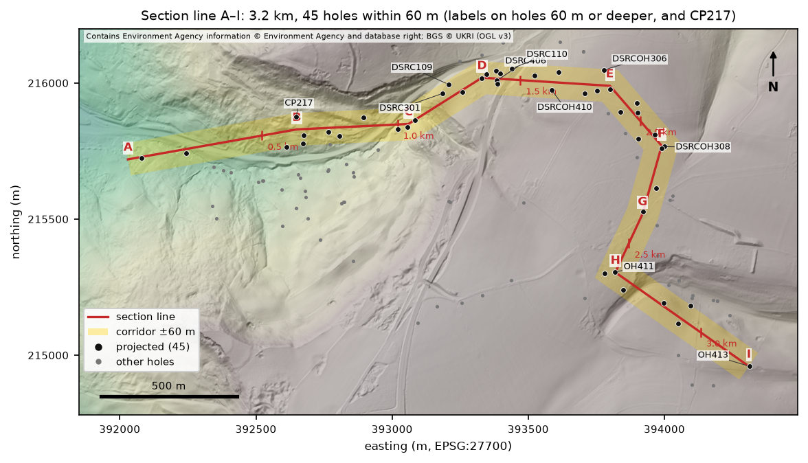
Shapely does the projection. line.project(point) gives the chainage of the nearest point on the line, and line.distance(point) how far the hole is from it. A small side() function adds a sign, so that holes to the left of the line looking from A have a positive offset:
holes = loca[["LOCA_TYPE", "LOCA_NATE", "LOCA_NATN", "LOCA_GL", "LOCA_FDEP"]].copy()pts = [Point(x, y) for x, y in zip(holes.LOCA_NATE, holes.LOCA_NATN)]holes["chainage"] = [line.project(p) for p in pts]holes["offset"] = [line.distance(p) * side(p, c) for p, c in zip(pts, holes.chainage)]on = holes[(holes.offset.abs() <= HALF) & (holes.LOCA_TYPE != "CPT")].sort_values("chainage").copy()=== Step 2: project the holes onto the section line ===section A-I: 8 legs, 3,217 m long | corridor ±60 m45 holes within 60 m (cone penetration tests left out: they have no GEOL descriptions) | 35 boreholes 10 m or deeper, 10 trial pits and shallow holes | 11 from Phase 2Adistance off the line: median 21 m, 21 within 20 m LOCA_TYPE LOCA_GL LOCA_FDEP chainage offsetLOCA_IDCP102 RC 127.6 20.0 51.0 -4.1CP200 RC 129.7 14.5 213.7 -14.3DSRC205 RC 167.2 30.0 581.5 -56.2CP217 RC 195.0 33.5 629.7 45.4CP210 RC 174.3 25.0 649.5 -54.0CP211 RC 183.4 35.0 652.8 -21.7...OH411 RC 280.5 101.0 2617.1 -1.3DSRC312 RC 282.2 25.1 2617.6 -40.5OH413 RC 270.6 100.4 3216.9 2.1A 60 m corridor is a compromise. Narrower, and the slope below the escarpment would have only two or three holes on it; wider, and holes on quite different parts of the hillside would be drawn side by side. Half the holes are within 21 m of the line, but some are more than 50 m off it, so the offset goes into the GeoPackage and into Figure 4 as evidence.
Step 3: sample the ground profile from LIDAR
The ground line comes from the same Environment Agency LIDAR composite DTM as Part 2, fetched at 2 m through the Defra WCS and cached as sixteen tiles. SciPy’s map_coordinates samples it bilinearly at a point every 2 m along the line, and again along lines either side of it, every 5 m out to the edge of the corridor:
ch = np.arange(0, line.length + STEP / 2, STEP)xy = np.array([line.interpolate(c).coords[0] for c in ch])ground = lidar(xy[:, 0], xy[:, 1])# Unit normal at every sample (left of the line), for the strip of ground across the corridor.d = np.gradient(xy, axis=0)normal = np.c_[-d[:, 1], d[:, 0]] / np.hypot(d[:, 0], d[:, 1])[:, None]across = np.stack([lidar(xy[:, 0] + o * normal[:, 0], xy[:, 1] + o * normal[:, 1]) for o in np.arange(-HALF, HALF + 1, 5)])lo, hi = across.min(axis=0), across.max(axis=0)=== Step 3: ground profile from Environment Agency LIDAR ===1,609 samples every 2 m: ground 121.0 to 281.0 m OD | steepest 20 m stretch 31 degacross the ±60 m corridor the ground varies by up to 34.4 m (median 13.0 m)LOCA_GL minus LIDAR at the hole: median -0.09 m, 43 of 45 within 0.5 mLOCA_GL minus the profile on the line: up to 15.5 m (CP210, 54 m off the line)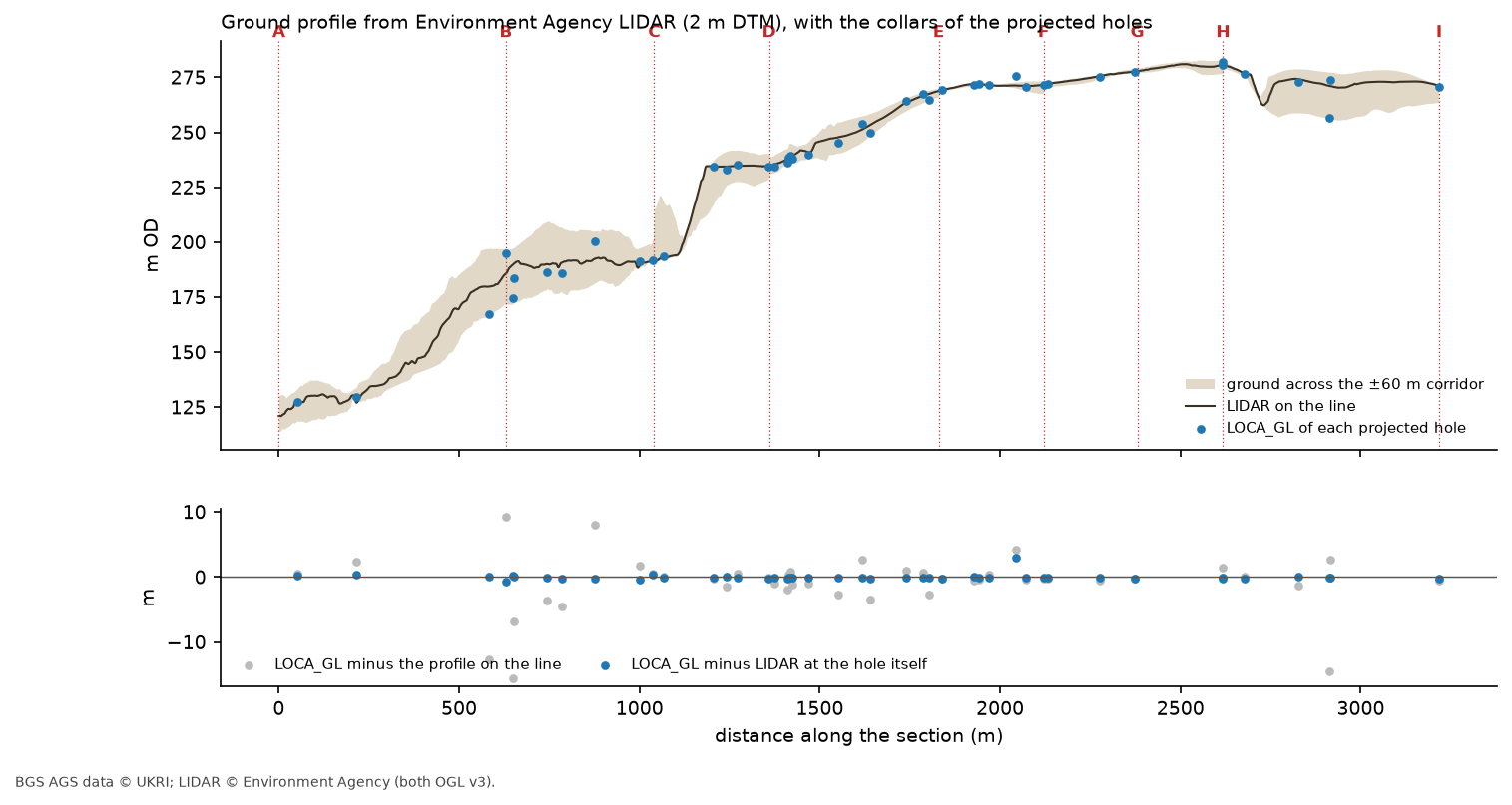
Two comparisons are worth keeping apart. At each hole itself, the recorded ground level agrees with LIDAR to a median of 0.09 m, as Part 2 found for the whole investigation. But compared with the ground on the line, a hole 54 m off it on the escarpment slope can be 15.5 m lower. Moving the log up to the line would invent 15 m of ground, so each log is drawn at its own ground level, and the buff band in the section shows how much the ground varies across the corridor. Where a log’s top sits away from the ground line, the band explains why.
Step 4: pick the contacts in each log
A contact is the boundary between two formations. The unit table in a417_ags.py gives each formation a rank by age, youngest first, so a contact can be found as the top of the first interval at or below a given rank, provided everything above it is younger:
SURFACES = pd.DataFrame([ ("FE", "top of Fuller's Earth", 3, "#2f6b2f"), ("IOG", "top of Inferior Oolite", 4, "#a0522d"), ("BDS", "base of Inferior Oolite", 7, "#111111"), ("WHM", "base of Bridport Sand", 8, "#1f4e9c"), ("MRB", "top of Marlstone Rock", 9, "#7a3b8f"),], columns=["key", "name", "rank", "colour"]).set_index("key")That works in most holes, but not in CP217. Part 1 found that its sequence repeats: Whitby Mudstone, Marlstone Rock and Dyrham Formation, and then from 19.10 m the same three again, which we read as a block of Lias that slid down the slope and rests on the sequence still in place. in_place() walks down the log and, if it meets a unit older than one it has already passed, starts again, so the contacts come from the lower sequence:
def in_place(g): """Bedrock intervals below any repeat in the sequence (CP217's slipped block), and the repeat's depth.""" rock = g[g["rank"] > 0] reached, split = 0, None for r in rock.itertuples(): if r.last < reached: split, reached = r.GEOL_TOP, 0 reached = max(reached, r.rank) return (rock if split is None else rock[rock.GEOL_TOP >= split]), split=== Step 4: pick the contacts in each log ===25 contacts picked in 20 holes (1 fall in a gap with no recovery, up to 0.90 m thick) holes lowest highestsurfacetop of Marlstone Rock 4 157.4 174.2base of Inferior Oolite 13 190.1 212.0base of Bridport Sand 2 193.9 195.5top of Fuller's Earth 3 254.0 270.6top of Inferior Oolite 3 231.4 274.8CP217: the sequence repeats from 19.10 m; contacts are taken from the lower, in-place sequencebase of the Inferior Oolite in 24 holes; more than 8 m from the median of their neighbours: RC507 (-13.9 m), RC508 (-11.2 m), RC509 (-15.2 m)The script also repeats Part 3’s neighbour test across both items, and it picks out the same three holes on top of Crickley Hill, RC507, RC508 and RC509, whose base of the Inferior Oolite is 11 to 15 m below the median of their neighbours. Their contacts are kept and drawn as red diamonds, but not used to draw the correlation lines.
What does projecting cost?
Moving a hole up to 60 m sideways onto the line moves its contacts too. To estimate by how much, the script fits a plane through the base of the Inferior Oolite in the other 21 holes and works out the change in height between each hole and its point on the line:
plane through 21 contacts: dip 1.3 deg towards 76 deg (bearing) | residuals RMS 7.8 m, largest 15.7 m (DSRC404)moving each contact from its hole to the line along that plane changes it by 0.14 m (median), 0.93 m at mostThe limestone dips gently east-north-east at about 1.3°, so moving the contacts the short distances involved here changes them by less than a metre. That is small next to the 3 m tolerance used in Step 5. The plane is only a rough fit, though: the residuals of up to 15.7 m show that the base of the limestone is not a simple flat surface even outside the three dropped holes.
Step 5: correlate the contacts and measure how much is inferred
Now the contacts are joined along the line, surface by surface. Two neighbouring contacts are joined only if they agree: within 3 m of each other, or no steeper between them than an apparent dip of 5°, which allows for the gentle regional dip over long gaps.
for key in SURFACES.index: c = contacts[(contacts.surface == key) & ~contacts.dropped].sort_values("chainage") for a, b in zip(c.itertuples(), c.iloc[1:].itertuples()): gap, dz = b.chainage - a.chainage, b.z - a.z agree = abs(dz) <= max(3.0, gap * tan_max) pairs.append(dict(surface=key, a=a.LOCA_ID, b=b.LOCA_ID, gap=round(gap), dz=round(dz, 1), agree=agree)) if agree: segments.append(dict(surface=key, c0=a.chainage, z0=a.z, c1=b.chainage, z1=b.z, style="solid" if gap <= SOLID_GAP else "dashed"))Lines between holes up to 150 m apart are drawn solid, and across wider gaps dashed. At each end, the surface is carried on at the plane’s apparent dip along that leg until it meets the ground, and drawn dotted:
=== Step 5: correlate the contacts and measure how much is inferred ===surface a b gap dz agree FE OH411 DSRC312 0 -3.1 False FE DSRC312 OH413 599 -13.6 True IOG RC516 OH411 244 -16.2 True IOG OH411 OH413 600 -27.1 True BDS DSRC301 DSRC109 38 0.3 True BDS DSRC109 DSRC302 115 -4.3 True BDS DSRC302 DSRC303 53 -2.4 True BDS DSRC303 DSRC406 3 -0.4 True BDS DSRC406 DSRC110 54 0.4 True BDS DSRC110 DSRCOH410 150 3.3 True BDS DSRCOH410 DSRCOH306 186 3.0 True BDS DSRCOH306 DSRCOH308 318 0.3 True BDS DSRCOH308 OH411 496 -17.7 True WHM DSRC301 DSRC109 38 -1.6 True MRB CP217 CP211 23 -16.8 False MRB CP211 CP214 91 13.3 False MRB CP214 CP215 40 -1.4 TrueThe base of the Inferior Oolite is the backbone of the section: with the three dropped holes set aside, all nine neighbouring pairs agree, the closest to within 0.3 m. Three pairs don’t agree, and each one tells us something:
- OH411 and DSRC312 are at the same chainage but 39 m apart across the line, and their top of the Fuller’s Earth differs by 3.1 m. That is just over the tolerance, and a fair measure of what projecting across a corridor can hide.
- CP217 and CP211 disagree by 16.8 m on the top of the Marlstone Rock, and CP211 and CP214 by 13.3 m. CP211’s Marlstone, at 157.4 m OD, is the odd one out: CP214 and CP215 agree with each other at about 170 m OD, and CP217’s in-place Marlstone is at 174.2 m OD. This is the landslipped slope below the escarpment, where Part 1 found CP217’s repeated sequence, so displaced blocks are what we’d expect.
The script then measures, for each surface, how much of the line drawn lies within 50 m of a logged contact, and how many neighbouring pairs agree:
near = (np.abs(xs[:, None] - cs[None, :]).min(axis=1) <= 50).mean() if len(xs) else np.nanhow much of each correlation line rests on a log: surface holes drawn_m between_close_holes_m across_wide_gaps_m carried_to_ground_m within_50m_of_a_log neighbours_agree top of Fuller's Earth 3 600 0 599 0.0 17% 1 of 2 top of Inferior Oolite 3 968 0 844 244.0 24% 2 of 2base of Inferior Oolite 10 1447 412 1000 60.0 47% 9 of 9 base of Bridport Sand 2 84 38 0 90.0 76% 1 of 1 top of Marlstone Rock 4 92 40 0 100.0 73% 1 of 3where each surface is carried up to the ground (chainage, m): top of Inferior Oolite 2129, base of Inferior Oolite 1145, base of Bridport Sand 1115, top of Marlstone Rock 530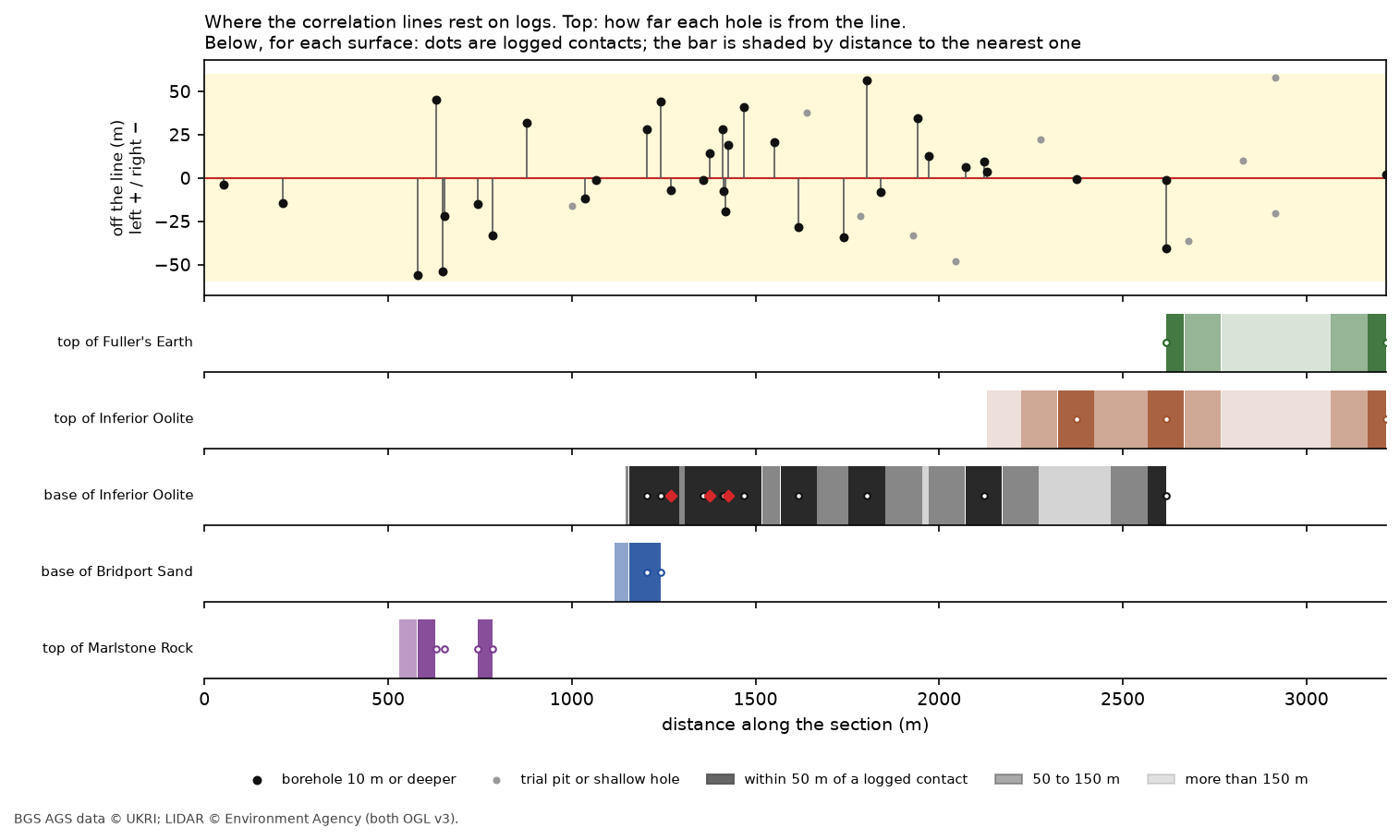
Read together, the table and Figure 4 show what the section is worth:
- The base of the Inferior Oolite rests on 10 logs over 1.4 km, with every neighbouring pair agreeing. It is the most reliable line on the section, and where it meets the ground at chainage 1,145 m it lies part-way up the steep face that the limestone forms in the LIDAR profile.
- The base of the Bridport Sand and the top of the Marlstone Rock are short, well-logged lines, but the Marlstone has only one agreeing pair out of three.
- The top of the Fuller’s Earth and the top of the Inferior Oolite on the plateau are mostly inferred: each rests on three holes up to 600 m apart. The lines are reasonable, since the beds dip gently east and each pair of holes is within the 5° allowance, but they are drawn across ground nobody has drilled.
Two close-ups: CP217 and the top of Crickley Hill
The full section is too long to show individual logs clearly, so the script draws two close-ups with less vertical exaggeration:
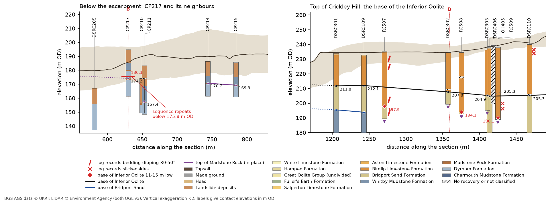
Below the escarpment (left), CP217’s upper Marlstone Rock is at 180.3 m OD and its in-place Marlstone at 174.2 m OD. The section supports Part 1’s reading of a slipped block resting on the sequence in place: the in-place contact is within 3.5 to 5 m of CP214 and CP215, 115 to 155 m further along, while the upper one is 10 m above them. CP211, only 23 m along the line but 67 m from CP217 across it, has the Marlstone 17 m lower still, so the slope here holds more than one displaced block, and the section leaves CP211 unjoined.
On top of Crickley Hill (right), the three dropped holes sit between holes that agree. RC508 is 18 m along the line from DSRC302 but 13.7 m lower; RC509 is 11 m from DSRC406 and 15 m lower. So whatever lowered them, the blocks are narrow, tens of metres across rather than hundreds. The logs carry the evidence Part 3 found: RC507 describes bedding dipping at 30 to 50° from near the surface into the Bridport Sand, and RC509 frequent slickensides between 36 and 43 m. That fits cambering and foundering, with narrow blocks of the limestone cap tilting and dropping into the soft Bridport Sand at the edge of the escarpment, better than a single fault, which would shift everything on one side of it. A small fault, or several, would still explain the drop, and the section can’t separate them; boreholes that can’t see the boundaries between blocks rarely can.
Step 6: the same section in QGIS
QGIS has had an elevation profile tool since version 3.26. It draws terrain, point clouds and 3D vector layers along any line, in a dock or as a print layout item. The script’s last step writes everything QGIS needs into one GeoPackage, together with the 2 m DTM clipped to the section and the ground profile as CSV:
# For the elevation profile, each interval is a 3D point at its base with an extrusion height equal to its thickness.iv = geol[geol.LOCA_ID.isin(on.index)]gpd.GeoDataFrame({"LOCA_ID": iv.LOCA_ID, "unit": iv.UNIT, "unit_name": iv.UNIT.map(A.UNITS.name), "colour": iv.UNIT.map(A.UNITS.colour), "top_mOD": iv.top_mOD.round(2), "base_mOD": iv.base_mOD.round(2), "thickness": (iv.top_mOD - iv.base_mOD).round(2), "GEOL_DESC": iv.GEOL_DESC}, geometry=[Point(r.LOCA_NATE, r.LOCA_NATN, r.base_mOD) for r in iv.itertuples()], crs="EPSG:27700").to_file(gpkg, layer="intervals", driver="GPKG")=== Step 6: write a GeoPackage for QGIS === section_line 1 LineString corridor 1 Polygon bends 9 Point holes 45 Point Z intervals 699 Point Z contacts 25 Point Zwrote output/a417_section.gpkg, a417_section_dtm_2m.tif (1440 x 830 cells) and ground_profile.csvWhy points rather than the vertical lines of Part 3? The elevation profile draws a 3D point as a marker at its z, but it can also extrude it upwards by a height taken from a field, which turns each interval into a vertical bar from its base to its top. Lines, by contrast, are drawn where they cross the profile curve, and a vertical line only touches it at one place.
qgis_section.py sets this up with PyQGIS. Run it with the Python that comes with QGIS, as in Parts 2 and 3:
"C:\Program Files\QGIS 3.40.12\bin\python-qgis-ltr.bat" qgis_section.pyThe key settings are in the layer’s elevation properties: absolute clamping so the z values are used as m OD, extrusion by the thickness field, and a profile line symbol coloured from the colour field:
ep = iv.elevationProperties()ep.setClamping(Qgis.AltitudeClamping.Absolute) # z is the base of the interval in m ODep.setExtrusionEnabled(True) # ... and the line rises by the interval's thicknessep.dataDefinedProperties().setProperty(QgsMapLayerElevationProperties.Property.ExtrusionHeight, QgsProperty.fromField("thickness"))ep.setRespectLayerSymbology(False)strip = QgsLineSymbol.createSimple({"width": "2.2", "capstyle": "flat"})strip.symbolLayer(0).setDataDefinedProperty(QgsSymbolLayer.Property.StrokeColor, QgsProperty.fromField("colour"))ep.setProfileLineSymbol(strip)Before building the layout, the script asks QGIS for its own ground profile along the section line with QgsProfileExporter, and compares it with the one cross_section.py sampled:
QGIS 3.40.12-Bratislava section_line valid=True features=1 corridor valid=True features=1 bends valid=True features=9 holes valid=True features=45 intervals valid=True features=699 contacts valid=True features=25 dtm valid=True 1440 x 830QGIS ground profile: 2022 points, 121.0 to 281.1 m OD | against ground_profile.csv: median |difference| 0.05 m, 95% within 0.32 msaved output/a417_section.qgz: 17 units in the profile (TOPS, SLIP, CHAM, MGR, NR, MRB, DYS, WHM, HEAD, BLPL, BDS, WHL, HMB, FE, SALS, ASLS, GOG)layout exported to output/_capture/06-qgis-section-layout.pngThe two profiles agree to a median of 0.05 m, and 95% of points to within a third of a metre. The small differences come from the two programs placing their samples slightly differently along the line. The script then builds an A4 print layout with a map frame above and an elevation profile item below. The profile item uses the section line as its curve with a 60 m tolerance, the same corridor as the Python version:
prof = QgsLayoutItemElevationProfile(layout)prof.setCrs(project.crs())prof.setProfileCurve(curve.clone())prof.setTolerance(HALF)prof.setLayers([dtm, layer["intervals"], layer["contacts"]]) # later layers draw on top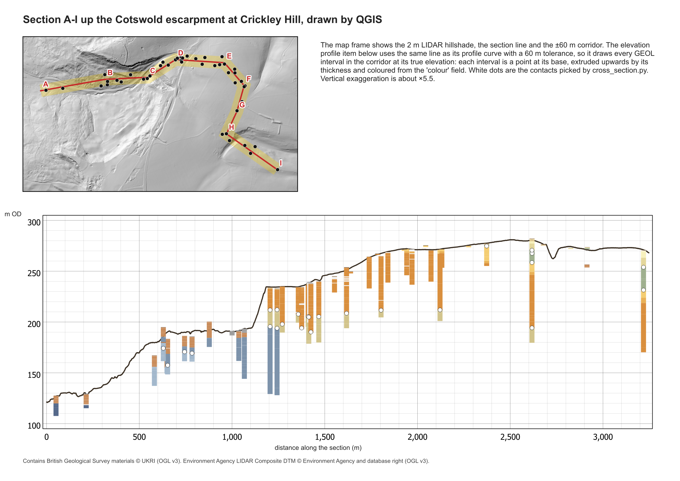
Open output/a417_section.qgz in QGIS Desktop to explore it interactively. Choose View > Elevation Profile, then Capture Curve from Feature and click the section line. Set the tolerance to 60 m to see the logs in the corridor. The interactive profile updates as you pan along it and can be exported as a 2D drawing or a CSV.
The QGIS version has no correlation lines: the elevation profile draws what is in the layers, and it doesn’t interpret. You could add the correlation lines as a LineStringZ layer of their own, but for a section that argues a case, the scripted matplotlib version gives you more control. The QGIS one is quicker to explore and keeps the section next to the map.
Frequently asked questions
How do I draw a geological cross-section from boreholes in Python?
Give each GEOL interval a top and base in m OD from LOCA_GL, choose a section line, and project each hole onto it with shapely’s line.project() to get its chainage. Draw each log as a stack of coloured rectangles at its chainage, sample a DTM along the line for the ground, and join the contacts between neighbouring holes. cross_section.py does all of this with matplotlib.
How wide should the corridor be?
Wide enough to catch the holes you need, but narrow enough that the ground and geology don’t change much across it. Measure both: here, the ground varies by a median of 13 m across a 120 m corridor, and the contacts change by under a metre when moved onto the line. Always draw each log at its own ground level rather than moving it to the ground on the line.
Can QGIS draw a geological cross-section?
QGIS 3.26 and later can draw borehole intervals and terrain along a line with the elevation profile tool, in a dock or a print layout. Store each interval as a 3D point at its base with its thickness as a field, enable extrusion by that field, and give the layer a profile line symbol coloured by unit.
Why use vertical exaggeration on a section?
The section is 3.2 km long but only about 170 m high, so at true scale the layers would be thin slivers. Five times exaggeration on the full section and twice on the close-ups make the logs readable. The trade-off is that slopes and dips look steeper than they are, so always state the exaggeration.
How do I show which parts of a section are inferred?
Use line styles that reflect the evidence: solid between close holes, dashed across wide gaps, dotted where a surface is projected beyond the last hole. Then measure, for each surface, how much of the line is within a set distance of a logged contact and how many neighbouring pairs agree, as Step 5 does.
Next steps
- Next in the series: Part 5: interpolated stratum surfaces such as rockhead, then Part 6: SPT N-values, and Part 7: a 3D-printed ground model.
- Kriging spatial interpolation in Python introduces the methods that turn contacts like these into continuous surfaces.
- Back to Part 1: Reading and validating AGS4 files, Part 2: Boreholes on a map or Part 3: 3D borehole logs.
Data and licences
- A417 Missing Link ground investigation (BGS deposited data item 173984; client Highways England, now National Highways; contractor Geotechnical Engineering Ltd) and A417 Missing Link ground investigation, Phase 2A (BGS deposited data item 173975; contractor Geotechnical Engineering Ltd), downloaded through the BGS AGS borehole index and export APIs. Contains British Geological Survey materials © UKRI 2026, licensed under the Open Government Licence v3.0.
- Environment Agency LIDAR Composite DTM 1 m, requested at 2 m from the Defra Data Services Platform WCS. © Environment Agency copyright and/or database right, licensed under the Open Government Licence v3.0. It gives the ground profile and the hillshade under every map in this post, and each figure carries the credit. No third-party web map tiles are used.
- Code:
cross_section.py,qgis_section.pyanda417_ags.py, tested with Python 3.12.0, python-ags4 1.2.0, GeoPandas 1.2.0, shapely 2.2.0, rasterio 1.5.2, SciPy 1.18.1, matplotlib 3.11.2 and QGIS 3.40.12.
Key terms
- Chainage
- Distance measured along a line from its start. On this section, a hole's chainage is the distance from A to the point on the line nearest the hole.
- Corridor
- A strip of fixed width either side of a section line. Holes inside it are projected onto the line; holes outside it are left off the section.
- Apparent dip
- The slope of a geological surface measured along a particular line, rather than in the direction it dips most steeply. It is never steeper than the true dip.
- Outcrop
- Where a geological surface meets the ground, whether or not it is visible at the surface.
- Foundering
- The sinking of blocks of hard cap rock into softer beds beneath, usually alongside cambering at the edge of an escarpment. Neighbouring blocks can end up at quite different levels.
- Elevation profile
- QGIS's tool for drawing terrain, point clouds and 3D vector layers along a line, in a dock or as a print layout item.
Data for this tutorial
- BGS AGS borehole data · Donated AGS ground investigation data, Open Government Licence
Licences and formats for each source are listed in the GIS data sources catalogue.