#Sentinel-2

24 posts

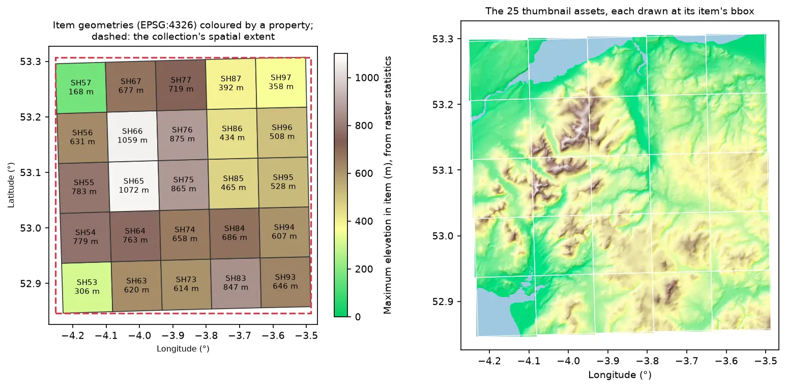
Two maps of Eryri in longitude and latitude. Left: 25 slightly rotated STAC item footprints labelled SH53 to SH97 and coloured by maximum elevation, inside a dashed red collection extent. Right: the 25 hillshaded thumbnail assets drawn at their item bounding boxes, forming one relief map

Tutorial Python Part 2 of 2

Build a STAC catalogue in Python with pystac, rio-stac and pystac-client

Turn 25 Cloud Optimised GeoTIFFs of Eryri into a static STAC catalogue with pystac and rio-stac, validate it against the JSON schemas, query it, serve it as static files, and compare it with the Earth Search and Planetary Computer STAC APIs through pystac-client.

Intermediate 12 min read

Tutorial Python

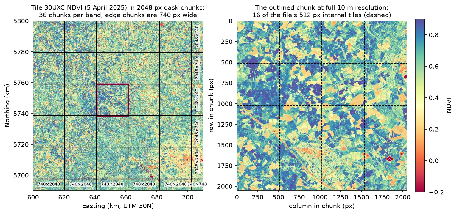
Parallel raster processing in Python with dask and rioxarray: a whole Sentinel-2 tile without running out of memory

Process large satellite rasters in Python with dask and rioxarray. Open eight full Sentinel-2 scenes lazily, choose a chunk size, inspect the task graph, watch CPU and memory with dask diagnostics, compare peak memory with eager NumPy, time chunk sizes and thread counts, and write a median NDVI GeoTIFF to disk chunk by chunk.

Intermediate 17 min read

Tutorial Python

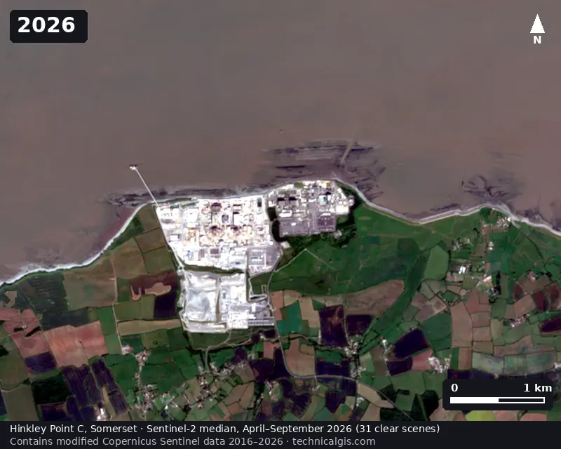
Satellite timelapse in Python: a Sentinel-2 GIF, WebP and MP4 of Hinkley Point C

Create a satellite timelapse in Python from free Sentinel-2 imagery. Select clear scenes with STAC, mask cloud, build one median composite per summer, apply a consistent stretch, add date labels and a scale bar, and export an animated GIF, WebP and MP4 of eleven years of construction at Hinkley Point C.

Intermediate 13 min read

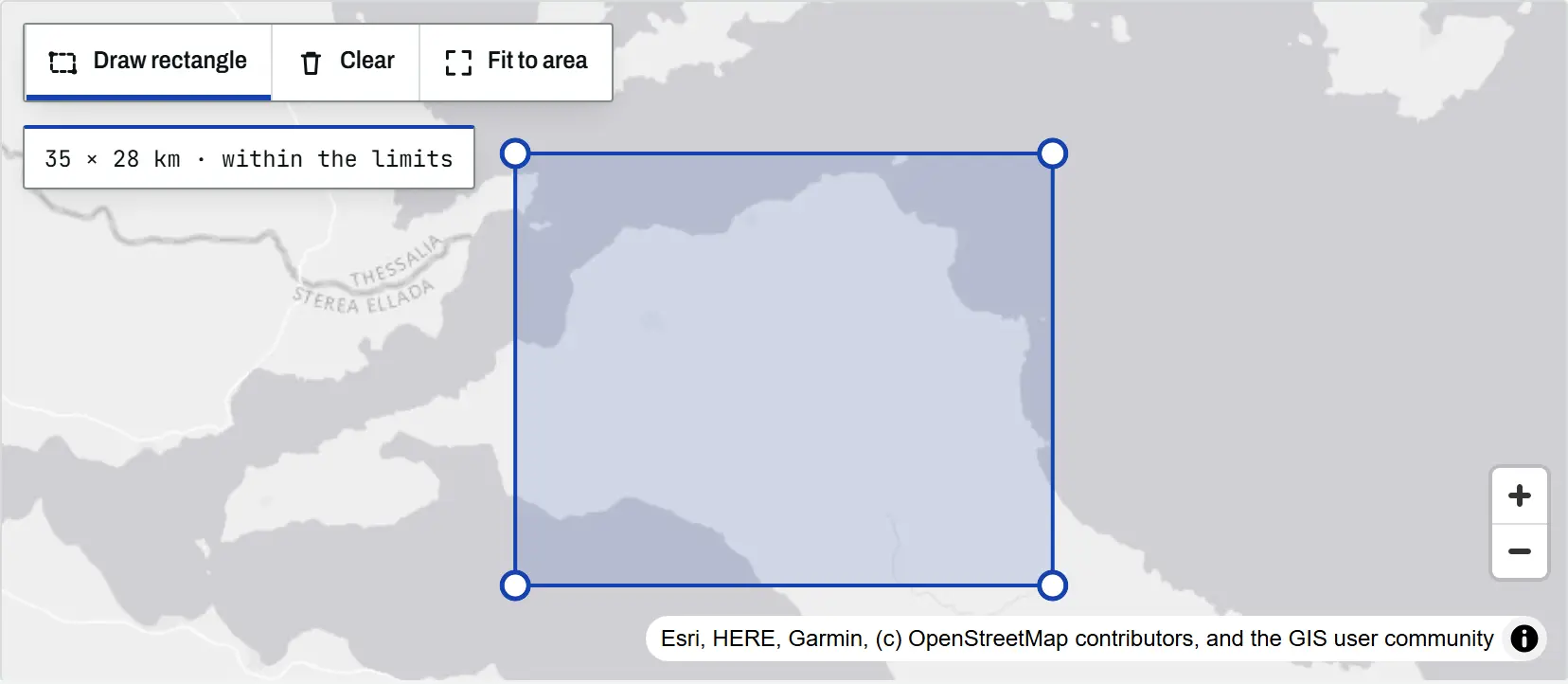
The climate tool map with a rectangle drawn over north Evia, Greece, its corner handles visible and a readout of 35 by 28 km within the limits

Article Remote Sensing

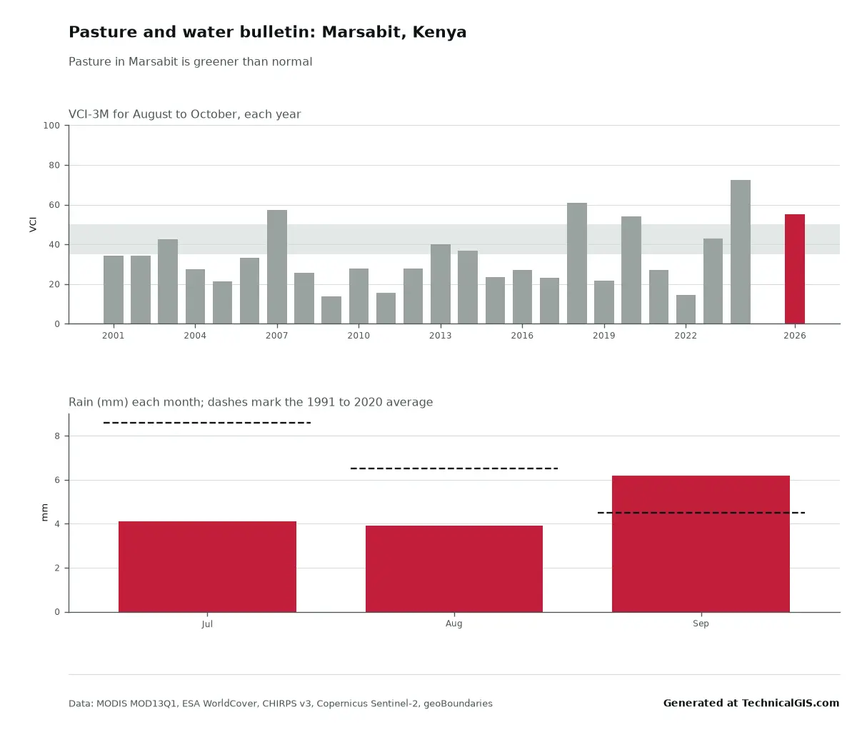
Climate time-series tools: charts and time-lapses for any place

An introduction to the TechnicalGIS climate time-series tools: five open datasets, how to draw an area on the map, worked examples from London, north Evia, Nairobi and Las Vegas, the processing limits and the terms for reusing every output.

Beginner 8 min read

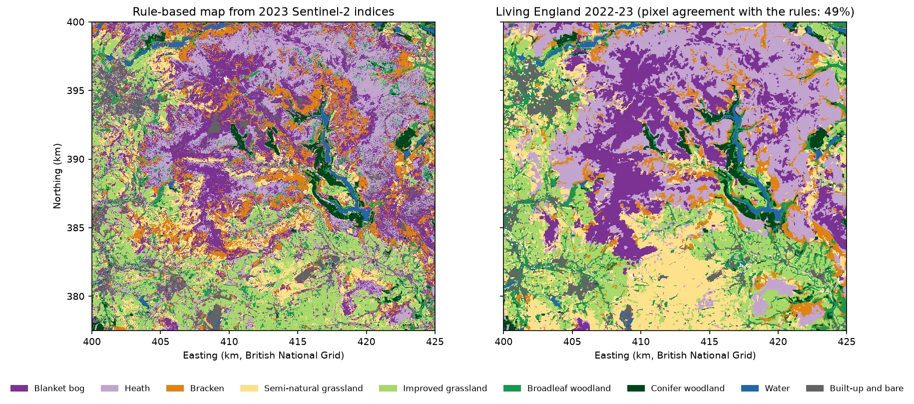
Two habitat maps of the Dark Peak side by side. Left: the rule-based map from Sentinel-2, with purple blanket bog and lilac heath on the Kinder and Bleaklow plateaux, orange bracken on the valley sides, green grassland and woodland in the valleys and blue reservoirs in the Derwent valley. Right: Living England 2022-23 for the same area, with smoother patches of the same classes.

Tutorial Python Part 1 of 5

Habitat mapping with Sentinel-2 in Python: spectral index rules and an honest accuracy assessment

Map blanket bog, heath, bracken, grassland, woodland, water and built-up land in the Peak District from 2023 Sentinel-2 seasonal composites with an eight-rule spectral index classifier, then assess it properly: a confusion matrix, user's and producer's accuracy, kappa and its caveats, block-bootstrap confidence intervals, and why a random train/test split overstates accuracy.

Beginner 19 min read

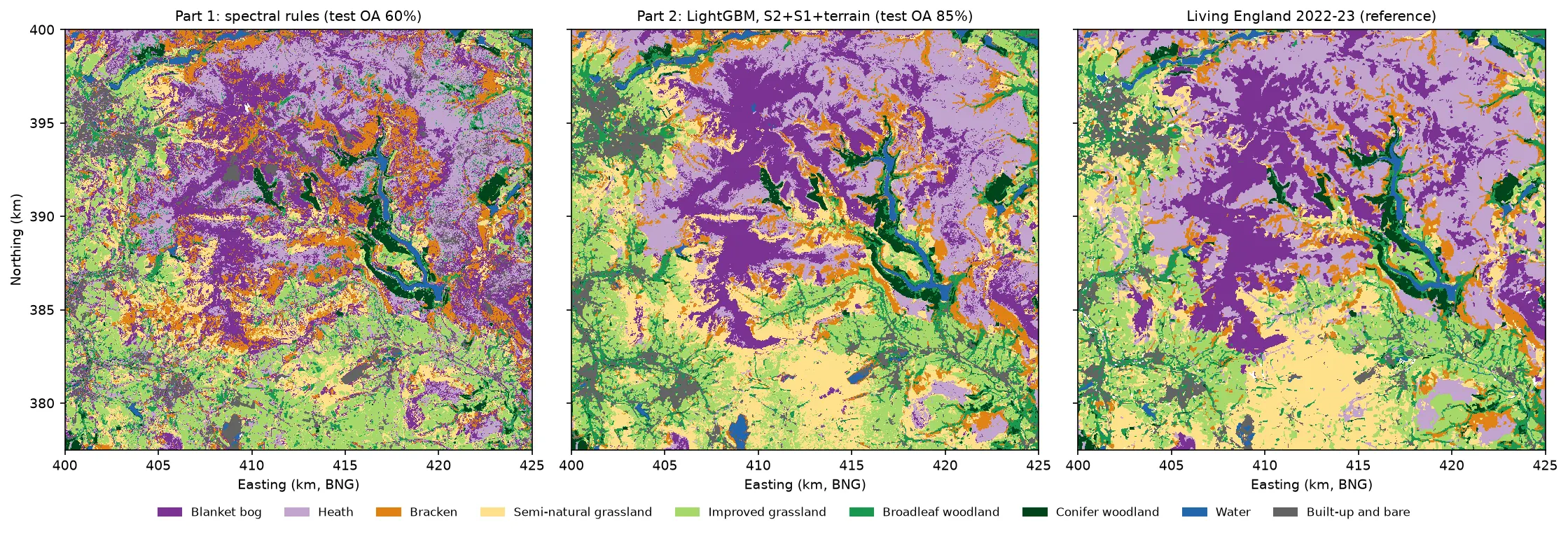
Three habitat maps of the Dark Peak side by side. Left: the noisy Part 1 rule-based map. Centre: the LightGBM map, with smooth purple blanket bog on the Kinder and Bleaklow plateaux, lilac heath around them, orange bracken on the valley sides, yellow semi-natural grassland in the south, green grassland and woodland in the valleys and blue reservoirs. Right: Living England 2022-23, which the LightGBM map closely resembles.

Tutorial Python Part 2 of 5

Habitat classification with LightGBM in Python: Sentinel-2, Sentinel-1 and terrain fusion

Classify nine upland habitats in the Peak District with LightGBM on 77 multi-temporal features: seasonal Sentinel-2 bands and indices, Sentinel-1 VV and VH backscatter and Copernicus DEM terrain. Tune with spatial-fold cross-validation and class weights, run an S2 / S2+S1 / S2+S1+terrain ablation, explain the model with TreeSHAP and permutation importance, and compare it with a random forest and the Part 1 rules on the same test blocks.

Intermediate 21 min read

Tutorial Python

Sentinel-2 cloud and cloud-shadow masking in Python: SCL vs s2cloudless vs OmniCloudMask

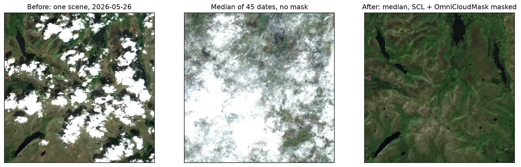
Mask clouds and cloud shadows in Sentinel-2 L2A imagery with Python. Compare the Scene Classification Layer (SCL), s2cloudless, OmniCloudMask and a simple threshold over the Lake District, measure how far they agree, score them against 186 reference points and build a cloud-free median composite.

Intermediate 15 min read

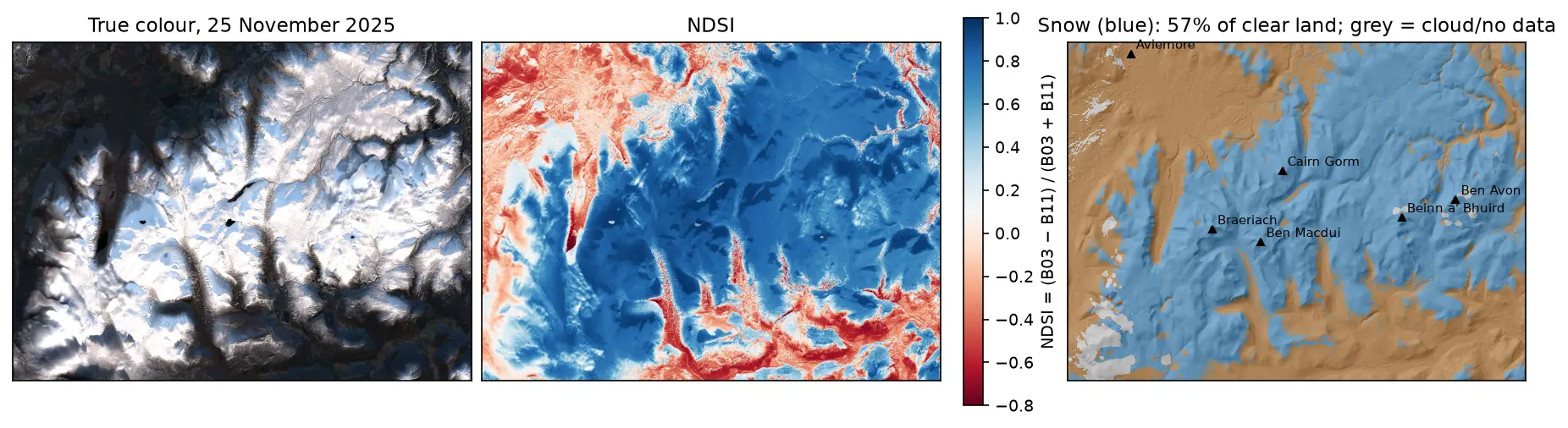
Three panels of the Cairngorms on 25 November 2025: a true-colour Sentinel-2 image with snow on the plateaux and long shadows in the glens; the NDSI, blue over snow and red over forest and bare ground; and a snow map over hillshade, with snow in blue on the high ground around Cairn Gorm, Ben Macdui, Braeriach, Beinn a' Bhuird and Ben Avon, covering 57% of the clear land.

Tutorial Python

Snow cover mapping with NDSI in Python: Sentinel-2 and MODIS over the Cairngorms

Map snow cover in Python with the Normalised Difference Snow Index (NDSI) from Sentinel-2 and the daily MODIS snow product on the Microsoft Planetary Computer: choosing the NDSI threshold, separating snow from cloud, snow-covered area through the winter of 2025–26 in the Cairngorms, and the snowline by elevation and aspect with the Copernicus DEM.

Intermediate 15 min read

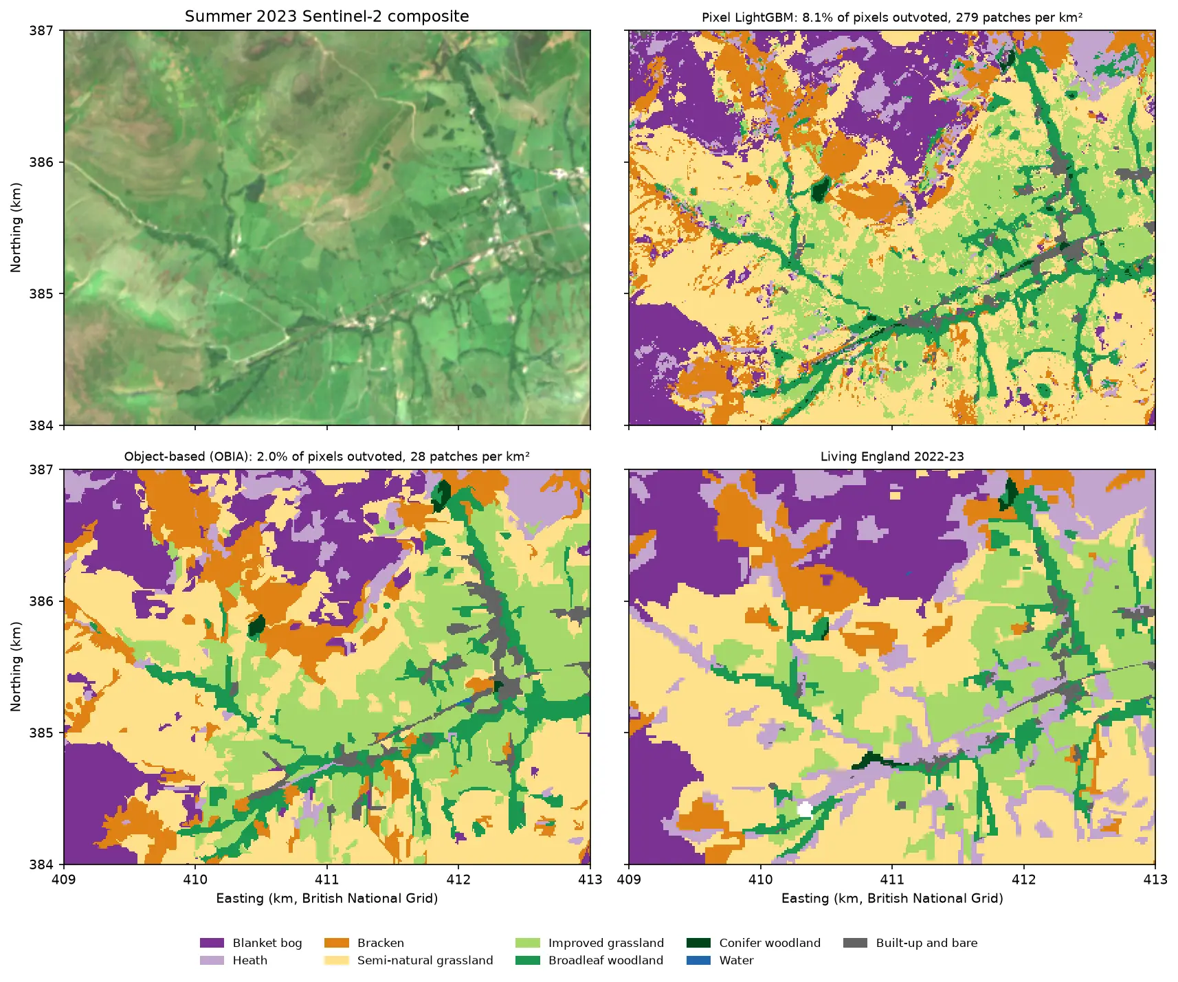
Four panels of the same 4 by 3 km area of the Edale valley and the southern edge of Kinder Scout. Top left: a true colour Sentinel-2 image of green fields and brown moorland. Top right: a pixel-based habitat map speckled with isolated pixels of other classes. Bottom left: the object-based map, with the same habitats in clean patches that follow field boundaries. Bottom right: the Living England reference map.

Tutorial Python Part 3 of 5

Object-based image analysis in Python: OBIA habitat classification with Sentinel-2

Segment 2023 Sentinel-2 seasonal composites of the Peak District into image objects with scikit-image SLIC and Felzenszwalb, tune the segment size against Living England boundaries, compute per-object statistics, shape and GLCM texture with NumPy, classify the objects with LightGBM and compare OBIA with a pixel-based classifier on accuracy, salt-and-pepper noise and patch counts. Then export the habitat objects as GeoPackage polygons.

Advanced 21 min read

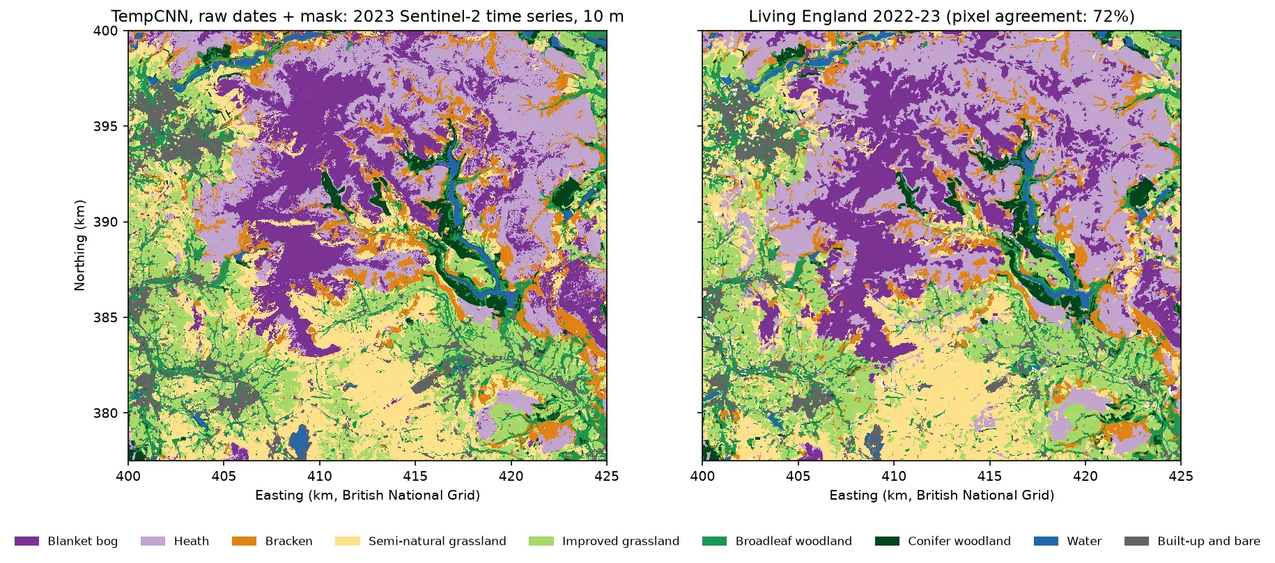
Two habitat maps of the Dark Peak side by side. Left: the TempCNN time-series map at 10 m, with purple blanket bog on the Kinder and Bleaklow plateaux, lilac heath around it, orange bracken on valley sides, yellow and green grassland in the south and west, dark green conifers and blue reservoirs in the Derwent valley. Right: Living England 2022-23 for the same area, which looks very similar but has more heath.

Tutorial Python Part 4 of 5

Satellite image time series classification with deep learning: TempCNN and L-TAE in PyTorch on a CPU

Classify habitats from a full year of cloudy, irregular Sentinel-2 observations with two temporal neural networks in PyTorch: a 1D convolutional TempCNN and a lightweight temporal attention encoder (L-TAE) with day-of-year positional encoding. Compare masking with gap-filling, test against a LightGBM baseline on spatial blocks, read which dates matter from attention and occlusion, and predict a wall-to-wall 10 m map on a CPU.

Advanced 24 min read

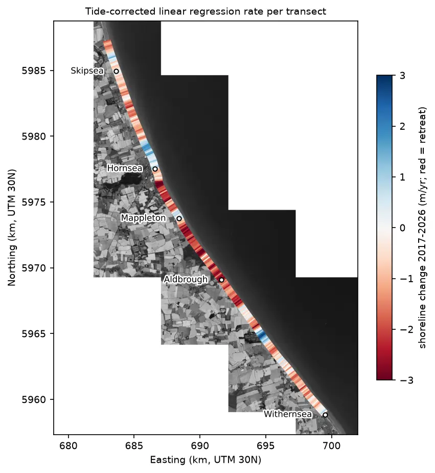
Map of the Holderness coast from Skipsea to Withernsea in greyscale Sentinel-2, with each 100 m transect coloured by its shoreline change rate from 2017 to 2026: mostly red (retreat), with blue (advance) patches north of Hornsea, at Mappleton and near Grimston.

Tutorial Python

Coastal erosion and shoreline change from Sentinel-2 in Python (Holderness, 2017–2026)

Measure shoreline change on one of Europe's fastest-eroding coasts with free Sentinel-2 imagery and Python: MNDWI and Otsu thresholding, sub-pixel shorelines with find_contours, shore-normal transects, a tide correction from open tide-gauge data, end-point and linear regression rates, and an honest comparison with East Riding of Yorkshire Council's cliff monitoring.

Advanced 21 min read

Tutorial Python

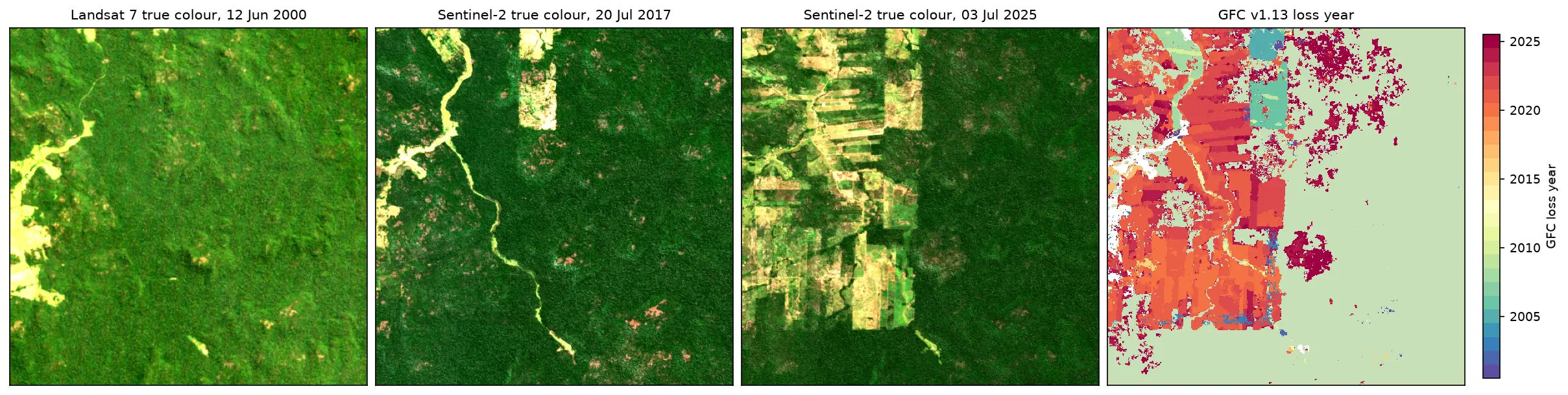
Deforestation detection in Python with Global Forest Change data (Rondônia, 2001–2025)

Map forest loss and deforestation in Python with the Hansen/UMD Global Forest Change v1.13 data: read the open tiles with no login, compute loss by year in hectares with correct pixel areas, compare Landsat and Sentinel-2 images before and after, and check the GFC loss year against Sentinel-2 NBR and MODIS burned area for central Rondônia, Brazil.

Intermediate 15 min read

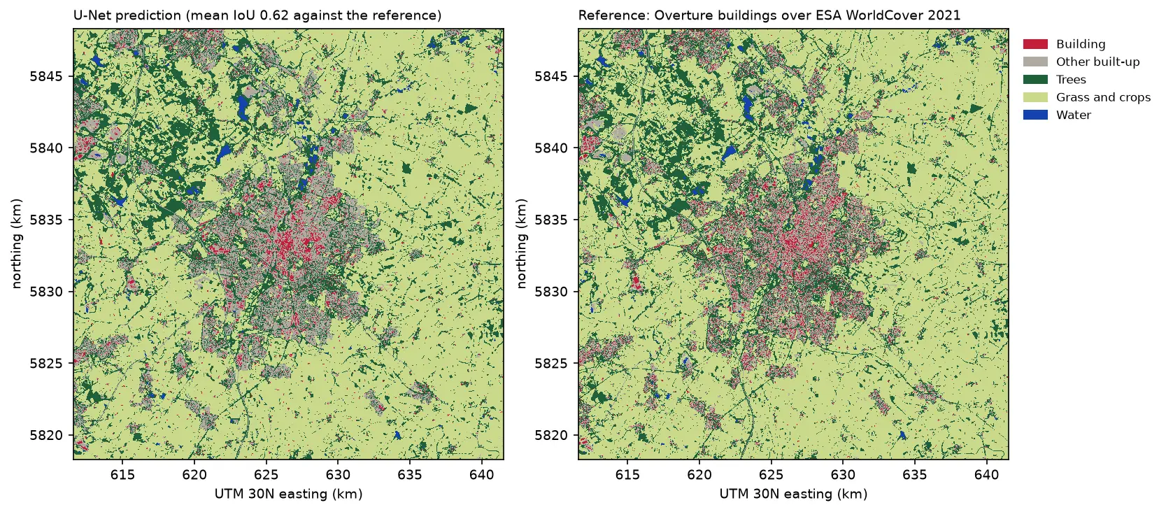
Two land cover maps of a 30 km square around Leicester side by side: the U-Net prediction on the left and the reference labels on the right. Both show the city in grey and red in the centre, surrounded by farmland in pale green, woods in dark green and reservoirs in blue. The prediction's city is smoother, with fewer separate red buildings.

Tutorial Python Part 3 of 3

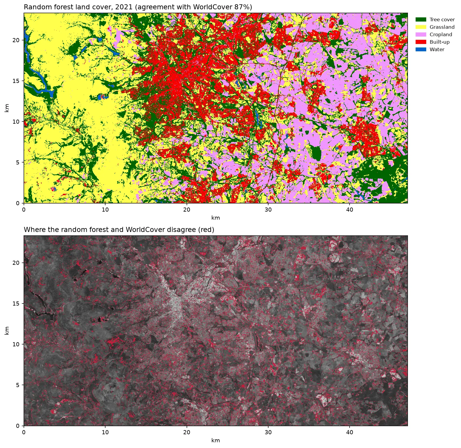
Deep learning inference on large rasters: sliding-window prediction, COGs and polygons in Python

Run a trained PyTorch U-Net over a whole Sentinel-2 scene of a city it has never seen: tiled sliding-window inference on a large GeoTIFF with overlapping, blended windows, a georeferenced Cloud Optimised GeoTIFF of classes and confidence, raster-to-vector polygons with rasterio.features.shapes in a GeoPackage, and an honest check against reference labels.

Advanced 13 min read

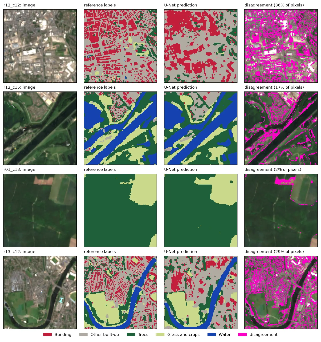
Four rows of Sentinel-2 test chips. Each row shows the image, the reference labels, the U-Net prediction and the disagreement in magenta. The prediction matches rivers, woods and fields closely, but in the city centre it draws buildings as blobs instead of separate roofs.

Tutorial Python Part 2 of 3

U-Net satellite image segmentation in PyTorch: a TorchGeo and Sentinel-2 tutorial on a CPU

Train a U-Net to segment Sentinel-2 imagery into buildings, built-up land, trees, grass and water with PyTorch, segmentation_models_pytorch and TorchGeo's Sentinel-2 pretrained ResNet-18 weights, on a CPU in five minutes. Real loss curves, per-class IoU and F1, a confusion matrix and an honest look at what limits accuracy.

Advanced 12 min read

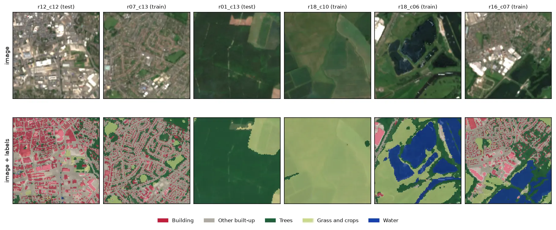
Six 128 by 128 pixel Sentinel-2 image chips of Nottingham, each shown above the same chip with its label mask overlaid: a city centre with red buildings and grey streets, a suburb, a forest, farmland, flooded gravel pits in blue and an industrial estate.

Tutorial Python Part 1 of 3

Training data for deep learning on satellite imagery: Sentinel-2 image chips in Python

Build a labelled deep learning dataset from free data: stream a Sentinel-2 L2A composite from the Planetary Computer, rasterise Overture building footprints over ESA WorldCover, cut georeferenced image chips, split them by spatial block so the test set does not leak, check the class balance and load it all as a TorchGeo dataset.

Intermediate 13 min read

Tutorial Python

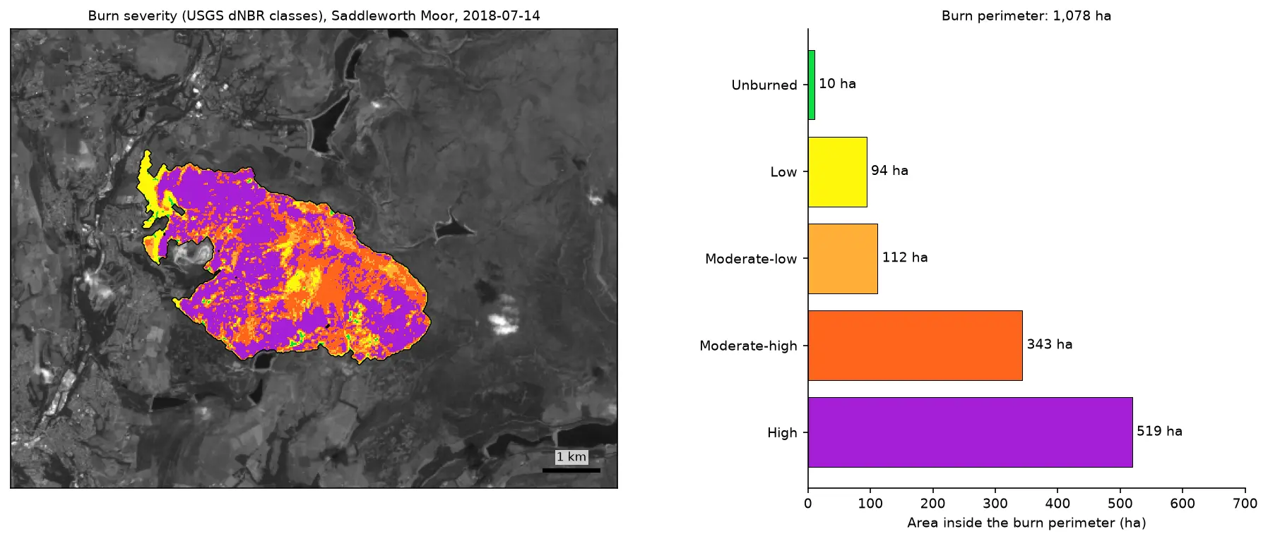
Burn severity mapping with Sentinel-2 and dNBR in Python (Saddleworth Moor 2018)

Map wildfire burn severity in Python with free Sentinel-2 imagery: NBR calculation, cloud and water masking with SCL, dNBR with an offset, USGS severity classes and burned hectares, a burn perimeter, fire progression, RdNBR and an eight-year recovery record for the 2018 Saddleworth Moor fire.

Intermediate 15 min read

Tutorial Python

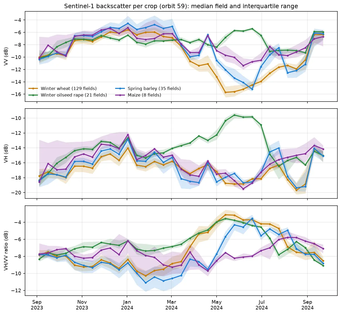
Sentinel-1 crop monitoring in Python: SAR time series for wheat and oilseed rape

Monitor crops through cloud with free Sentinel-1 radar. Build VV, VH and VH/VV ratio time series for 247 fields in Cambridgeshire, beat speckle by field-averaging, read the growth signatures of winter wheat and oilseed rape, and compare with the gaps that cloud leaves in Sentinel-2 NDVI.

Intermediate 16 min read

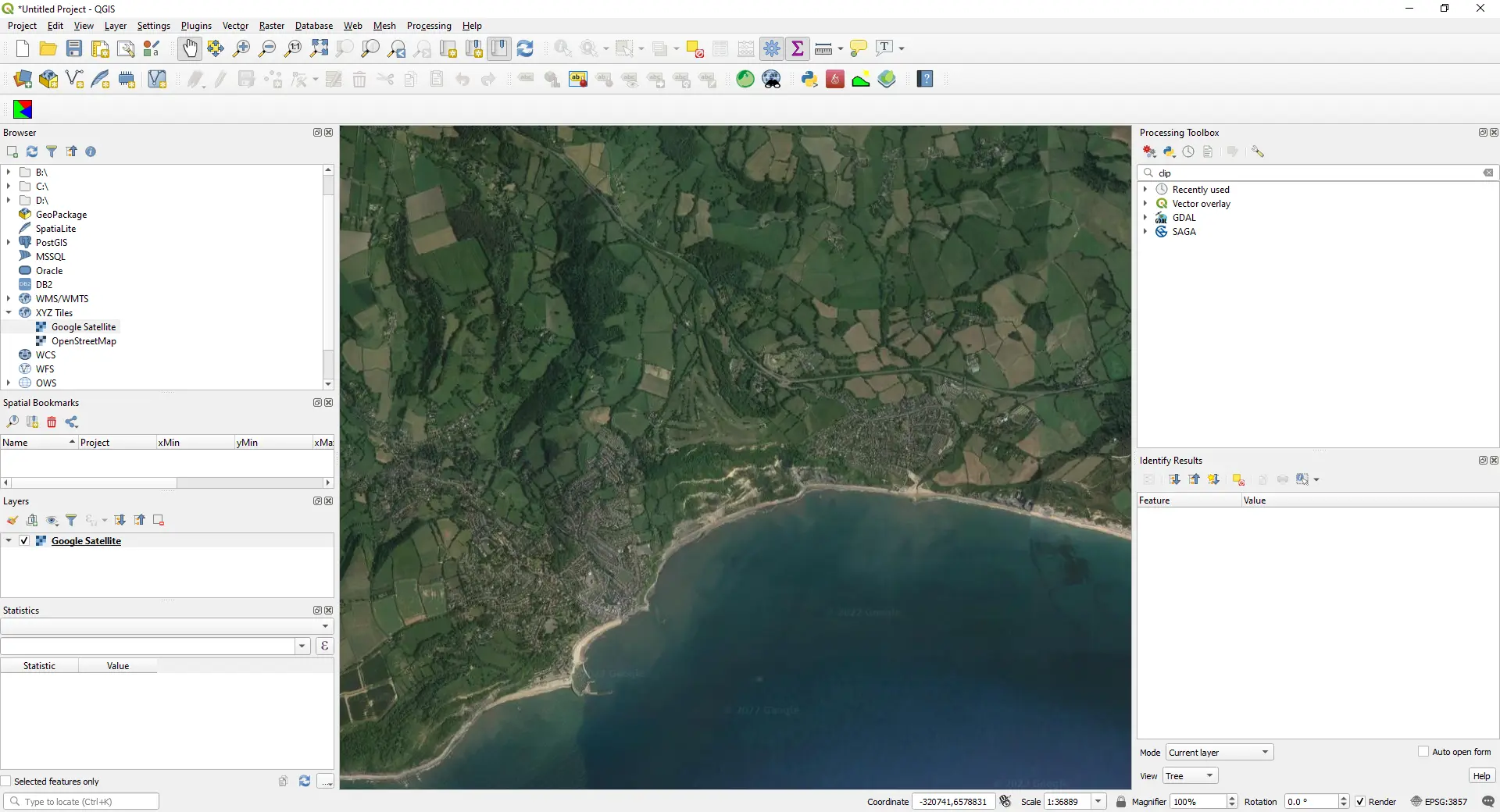
QGIS map window showing Google satellite imagery of a stretch of the south coast of England, loaded as an XYZ Tiles layer (screenshot from the original 2022 version of this post).

Article QGIS

How to Add Google Maps and OpenStreetMap Layers to QGIS

Add OpenStreetMap, satellite and Google basemaps to QGIS 3.40 LTR, 3.44 and 4.x as XYZ Tiles connections: the correct tile URLs, the OpenStreetMap tile usage policy, the licence-safe ways to get Google, Esri and Sentinel-2 imagery, and the same basemaps from PyQGIS, folium, leafmap and contextily.

Beginner 13 min read