3D-print a geological ground model: one watertight STL per stratum

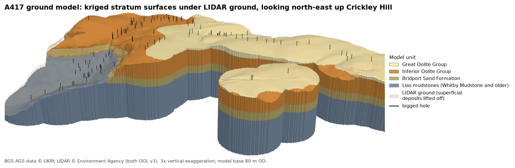
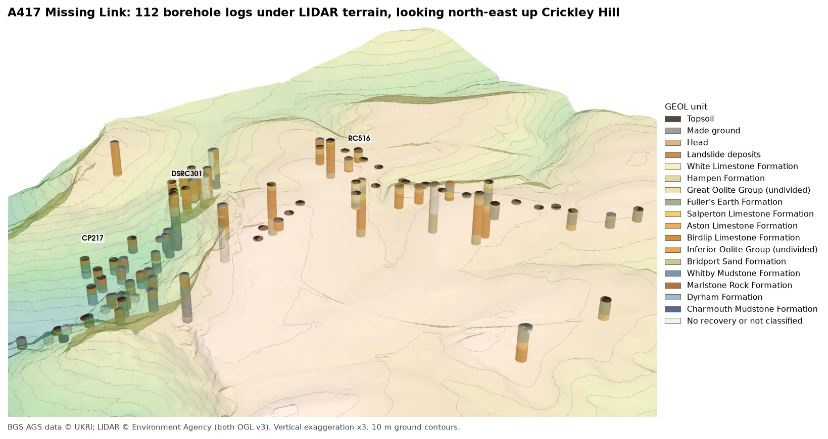
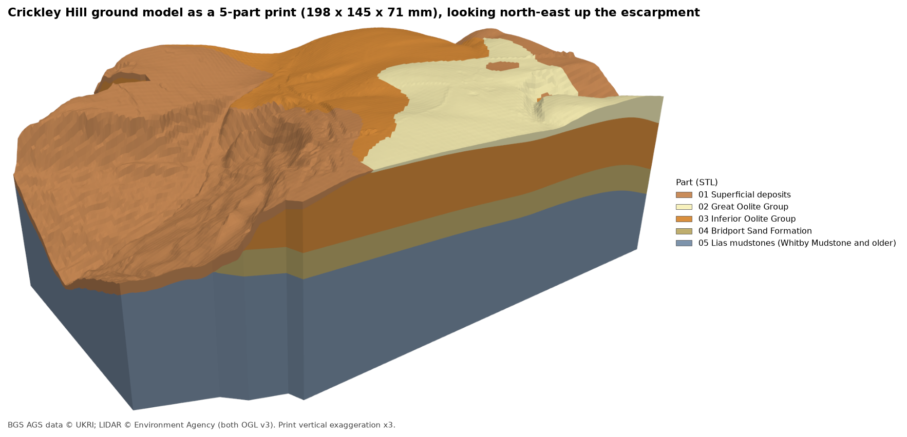
A ground model you can hold in your hand explains a site faster than any section. In Part 5 we kriged the A417 boreholes into a stack of stratum surfaces under the LIDAR ground, and tested them. Now we print them: a 20 cm block of the Cotswold escarpment at Crickley Hill, with the superficial deposits, Great Oolite, Inferior Oolite, Bridport Sand and Lias each printed as a separate part in its own colour.

The approach is the one from the 3D-printed maps with Python series: build one watertight solid per colour with mesh booleans, check every part, and write STLs and a 3MF. What is new is that the colours are not drawn on the surface; they are the geology, and they go all the way through. Cut the print in half and you see the section.

The steps are:

1. read the stratum surfaces in the print window;
2. trace the footprint of the model;
3. convert to print heights, and decide what is too thin to print;
4. build one solid per unit;
5. check every part before writing;
6. write one STL per unit and a colour 3MF;
7. render the previews from the STL files.

The code is print_ground_model.py. It reads output/model/ from Part 5 and runs in about seven seconds.

Step 1: the stratum surfaces in the print window

Part 5 wrote each surface as a GeoTIFF on the same 10 m grid, plus a model.json listing the units from the top down. The top of each unit is the base of the one above, and the bottom unit runs down to a flat model base at 80 m OD. The script checks that before it reads anything, so a change to Part 5 that broke the stack would stop here, not in the slicer.

meta = json.loads((args.model / "model.json").read_text(encoding="utf-8"))
units, base_m = meta["units"], float(meta["model_base_mOD"])
for upper, lower in zip(units, units[1:]):
    assert upper["base"] == lower["top"], f"{upper['code']} base and {lower['code']} top must be the same surface"
assert units[-1]["base"] is None, "the bottom unit runs down to the flat model base"

grids = []
for u in units:
    with rasterio.open(args.model / f"{u['top']}.tif") as src:
        win = from_bounds(*WINDOW, transform=src.transform).round_offsets().round_lengths()
        win = win.intersection(Window(0, 0, src.width, src.height))
        grids.append(src.read(1, window=win).astype("float64"))
        res, wt = src.res[0], src.window_transform(win)
S = np.stack(grids)                                   # (surface, row, col), top surface first
valid = np.isfinite(S).all(axis=0)

The window, 1.9 by 1.4 km, takes in the scarp face, the plateau and the vale below, where the boreholes are densest. Part 5 only modelled ground within 300 m of a logged hole, so the model covers 89.6% of the window.

Part 5 already made sure the surfaces never cross, but a print is unforgiving, so the script applies the rule again (np.minimum.accumulate down the stack) and counts how many cells it had to change. None did:

=== Step 1: read the stratum surfaces in the print window ===
window 392400-394300 E, 215000-216400 N: 190 x 140 cells of 10 m | model domain covers 89.6% of it
5 units, model base 80 m OD | cells needing re-clamping 0, below the model base (raised to it) 0
  top of SUP   Superficial deposits        134.0 to  295.4 m OD
  top of GOG   Great Oolite Group          127.8 to  294.3 m OD
  top of IOG   Inferior Oolite Group       127.8 to  293.1 m OD
  top of BDS   Bridport Sand Formation     127.8 to  238.7 m OD
  top of LIAS  Lias mudstones (Whitby Mudstone and older)  127.8 to  212.6 m OD

Where a unit has been eroded away, its top and base are the same surface. That is why so many units share a minimum of 127.8 m OD: down in the vale they all have zero thickness on top of the Lias.

Step 2: the footprint

The print follows the edge of the model, not the rectangle of the window. Each mesh vertex sits at a cell centre, so a grid square only holds real data if all four of its corners are valid. The script turns those squares into a polygon, pulls the edge in by one cell and simplifies it by no more than that. This gives clean straight walls instead of a pixel staircase, without ever reaching outside the modelled ground:

scale = LONG_MM / ((max(rows, cols) - 1) * res)      # mm on the print per metre on the ground
cell = res * scale
quad = valid[:-1, :-1] & valid[1:, :-1] & valid[:-1, 1:] & valid[1:, 1:]
quad_to_mm = rasterio.Affine(cell, 0, 0, 0, -cell, (rows - 1) * cell)
foot = unary_union([shape(g) for g, _ in features.shapes(quad.astype("uint8"), mask=quad, transform=quad_to_mm)])
foot = foot.buffer(-cell, join_style="mitre").simplify(cell)
pieces = sorted(getattr(foot, "geoms", [foot]), key=lambda g: g.area, reverse=True)
foot = orient(pieces[0], 1.0)                         # outer ring anticlockwise, holes clockwise

=== Step 2: the footprint of the model domain ===
horizontal scale 1:9,450 | one 10 m cell = 1.06 mm on the print
footprint 2.28 km2 = 255.3 cm2 on the print, 0 hole(s) | 0 smaller piece(s) left out (0 m2)

A 10 m cell is 1.06 mm on the print, about two and a half nozzle widths, so a 0.4 mm nozzle can show every cell of the grid.

Step 3: print heights, and what is too thin to print

First the scale. The print is 200 mm on its long side, so 198 by 145 mm fits a common 220 mm build plate with room for a brim, and a 10 m cell is 1.06 mm: two and a half nozzle widths. Heights become millimetres above the print bed: metres above the model base, times the scale, times a vertical exaggeration of three, on top of a 3 mm plinth. Three times is the exaggeration of the 3D views in Parts 3 and 5, so the print matches the pictures. It makes the Bridport Sand a clear 9 mm band and keeps more of the superficial deposits, while the scarp still reads as a slope rather than a cliff.

Then comes the most important decision in the script. A layer thinner than about three print layers will not print as a recognisable band: the slicer either drops it or prints a speckle of one colour over another. So any unit thinner than MIN_MM = 0.6 mm in a cell is handed to the unit below. The script raises that unit’s base up to its top, so the next real unit down fills the space:

Z = (S - base_m) * scale * VE + BASE_MM
for k, u in enumerate(units[:-1]):
    t = Z[k] - Z[k + 1]
    thin = (t > 1e-6) & (t < MIN_MM)
    old = Z[k + 1].copy()
    for j in range(k + 1, len(units)):
        Z[j] = np.where(thin & (Z[j] >= old - 1e-9), Z[k], Z[j])

The inner loop matters where units have been eroded. If the Great Oolite is absent, its base is the same surface as the top of the Inferior Oolite, so both are raised together and the Inferior Oolite takes the space.

=== Step 3: print heights, vertical exaggeration x3, nothing thinner than 0.6 mm ===
1 m of ground = 0.317 mm on the print, so 0.6 mm = 1.89 m of strata
SUP   present under  96.0% of the footprint | thinner than 0.6 mm under  48.5% (1,094,700 m2) -> absorbed by the unit below
GOG   present under  26.1% of the footprint | thinner than 0.6 mm under   1.4% (32,400 m2) -> absorbed by the unit below
IOG   present under  75.6% of the footprint | thinner than 0.6 mm under   0.4% (8,200 m2) -> absorbed by the unit below
BDS   present under  80.9% of the footprint | thinner than 0.6 mm under   0.6% (12,800 m2) -> absorbed by the unit below

At this scale 0.6 mm is 1.89 m of ground. The bedrock units are almost all thicker than that, and lose at most 1.4% of the footprint. The superficial deposits are different: they are present almost everywhere, but over much of the plateau they are a metre or so of topsoil and weathered stone (the median logged thickness is 1.0 m). They are thinner than 1.89 m under 48.5% of the footprint, so about half their area prints in the colour of the rock beneath and half survives. What stays is the thick head and landslide debris on the scarp slope and the deeper patches on the plateau, which is what an engineer would want to see. For comparison, a 160 mm print at twice exaggeration would have lost 62% of their area.

Step 4: one solid per unit

Each unit is built from two heightfield solids, using the same heightfield_solid helper as the multi-colour terrain print. cum[k] runs from the bottom of the plinth up to surface k, so unit k is cum[k] minus cum[k + 1]. The footprint is extruded into a prism and intersected with each part:

prism = mf.Manifold.extrude(mf.CrossSection(contours), float(Z.max()) + 2).translate((0, 0, -1))
cum = [to_manifold(*heightfield_solid(z, cell)) for z in Z]      # plinth bottom up to each surface
raw = [(cum[k] - cum[k + 1]) ^ prism for k in range(len(units) - 1)] + [cum[-1] ^ prism]
whole = cum[0] ^ prism
solids = {}
for u, m in zip(units, raw):
    solids[u["code"]], n = drop_slivers(m)

The order of the operations matters. If you trim each solid to the footprint first and subtract afterwards, every solid has the same side walls, and subtracting two coincident walls leaves needle-thin triangles on the outside of the print. Subtracting first and trimming last cuts all the side walls in one clean operation.

Where two surfaces touch, as they do wherever a unit thins to zero, the booleans can leave zero-volume slivers. drop_slivers splits each result into connected pieces and keeps only those over 0.05 mm³:

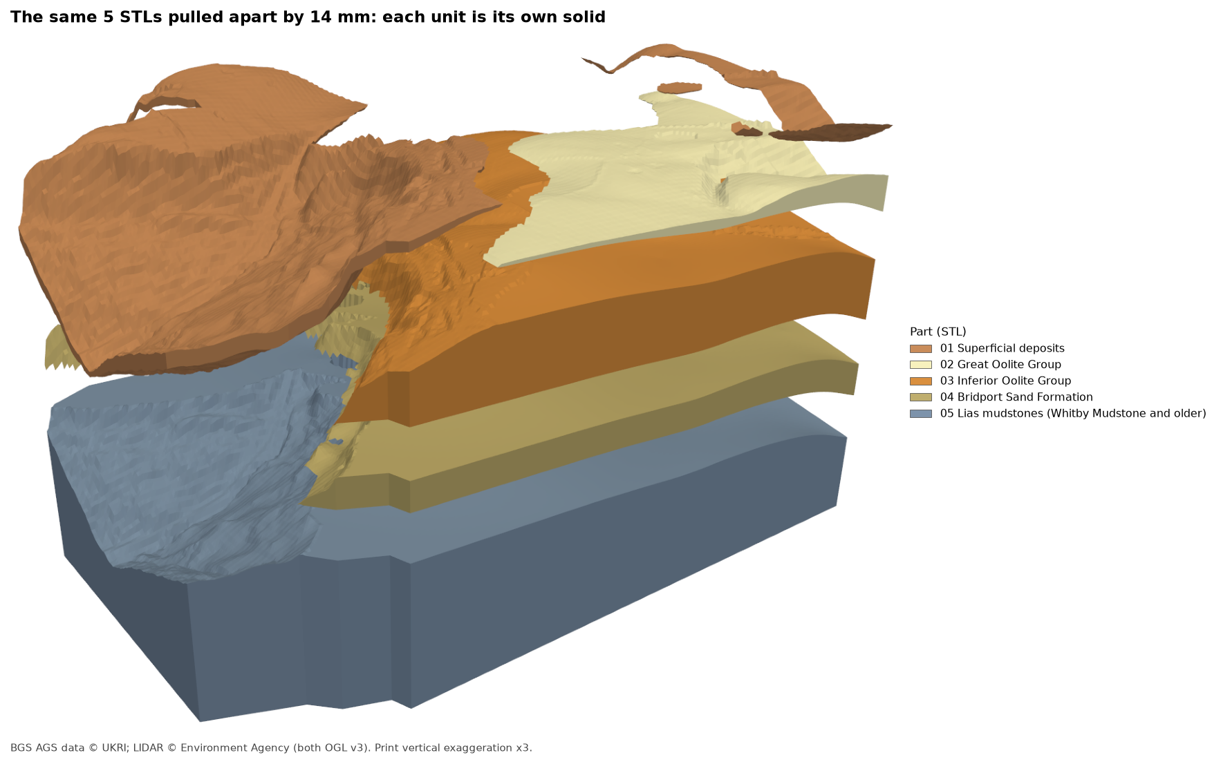
=== Step 4: cumulative solids and booleans ===
whole model 197.9 x 145.0 x 71.4 mm, including the 3 mm plinth
SUP     4 separate piece(s)
GOG     1 separate piece(s)
IOG     1 separate piece(s)
BDS     1 separate piece(s)
LIAS    1 separate piece(s)

The superficial deposits are in four pieces: the large spread on the scarp slope, a strip along the north-eastern edge of the plateau and two small patches on it. All four are real deposits thicker than 1.89 m.

Step 5: check every part before writing

Nothing is written until every part passes. check_mesh counts edges: in a watertight mesh every edge is shared by exactly two triangles, and in a consistently oriented one each edge is used once in each direction. It also works out the volume from the triangles, which must be positive (a negative volume means the mesh is inside out):

def check_mesh(verts, tris):
    """Every edge shared by exactly two triangles, used once in each direction, and a positive volume."""
    e = np.concatenate([tris[:, [0, 1]], tris[:, [1, 2]], tris[:, [2, 0]]])
    n = len(verts)
    und = np.unique(np.sort(e, axis=1) @ np.array([n, 1]), return_counts=True)[1]
    drc = np.unique(e @ np.array([n, 1]), return_counts=True)[1]
    t = verts[tris]
    vol = np.einsum("ij,ij->i", t[:, 0], np.cross(t[:, 1], t[:, 2])).sum() / 6
    return bool((und == 2).all()), bool((drc == 1).all()), vol

Then the parts are checked against each other. Their volumes must add up to the whole ground solid, and no two parts may share any volume. If either test fails, the script stops:

total, whole = sum(m[2] for m in meshes.values()), whole.volume()
overlap = sum((solids[a] ^ solids[b]).volume() for i, a in enumerate(codes) for b in codes[i + 1:])
if abs(total - whole) > 0.001 * whole or overlap > 0.001 * whole:
    raise RuntimeError("the parts do not add up to the ground solid")

=== Step 5: check every part before writing ===
sum of parts 1450.952 cm3 | ground solid 1450.952 cm3 | difference +0.0000% | pairwise overlap 0.0000 mm3

The parts fill the model exactly, with nothing missing and nothing printed twice.

Step 6: one STL per unit and a colour 3MF

Each part is written as a binary STL with the structured-dtype writer from DEM to STL, numbered from the top down so they sort in order in the slicer. All five also go into one 3MF, with the unit names and the same colours as Part 5’s figures:

=== Step 6: write one STL per unit and a colour 3MF ===
file           unit                       triangles     cm3  PLA g  watertight
01_SUP.stl     Superficial deposits          46,676   35.62   44.2  True
02_GOG.stl     Great Oolite Group            24,120   23.63   29.3  True
03_IOG.stl     Inferior Oolite Group         72,058  305.67  379.0  True
04_BDS.stl     Bridport Sand Formation       76,698  172.61  214.0  True
05_LIAS.stl    Lias mudstones (Whitby Mudstone and older)    93,058  913.43 1132.6  True
total                                       312,610 1450.95 1799.2  (solid PLA; at 15% infill a slicer will use much less)
ground_model.3mf 2.9 MB | 5 parts: Superficial deposits, Great Oolite Group, Inferior Oolite Group, Bridport Sand Formation, Lias mudstones (Whitby Mudstone and older)

The volumes are for solid parts. With two or three walls and 15% infill, the Lias block uses a fraction of its 1.1 kg, and the thin upper parts are mostly wall anyway. If you want to save more, raise the model base in Part 5: everything below the lowest surface, 127.8 m OD, is plain Lias plinth.

Step 7: previews from the STL files

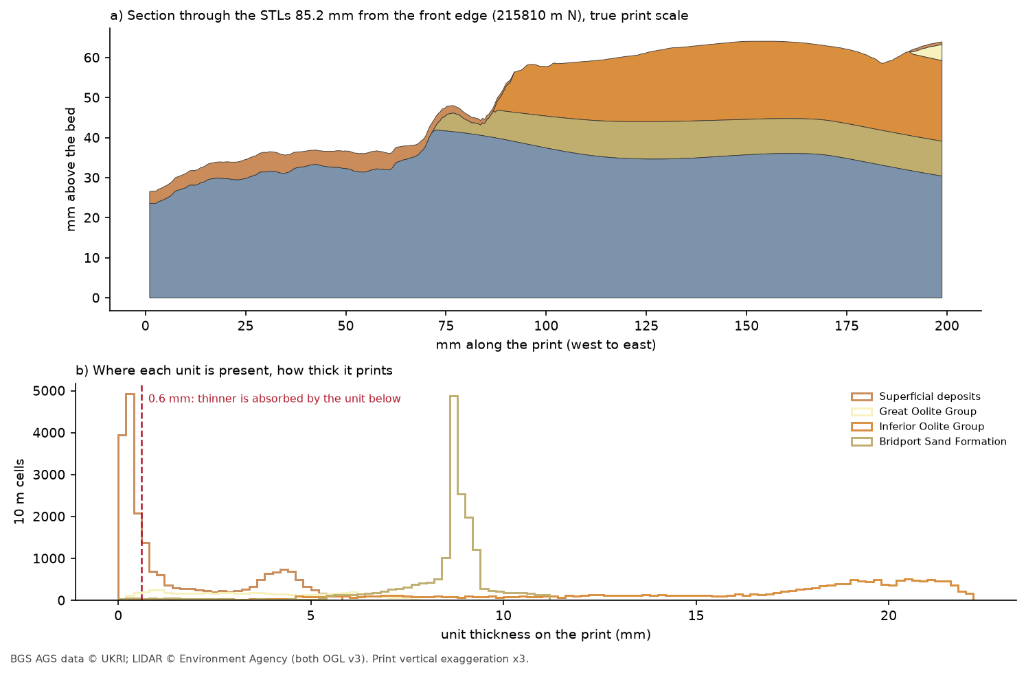
Every picture in this post is rendered from the STL files read back from disk with pv.read, not from the arrays in memory. If the files were wrong, the pictures would be too. The section in figure 3 is cut through the STL meshes with manifold3d’s slice.

=== Step 7: previews rendered from the STL files ===
read back 5 STLs: 197.9 x 145.0 x 71.4 mm
figures written: 01-printable-ground-model.png, 02-exploded-view.png, 03-print-layers-section.png, 04-slicer-style-top.png
finished in 6.9 s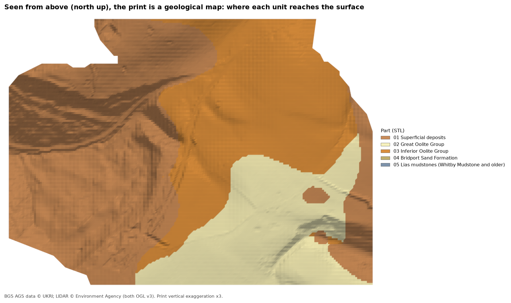

Printing tips

• Loading the parts: drag all five STLs into PrusaSlicer, Bambu Studio or OrcaSlicer together and accept the offer to load them as one object with multiple parts, so they stay aligned. Or open ground_model.3mf, which keeps the names and positions. Then give each part its filament.
• Colours: follow the geological map if you can: a brown or tan for superficial deposits, cream for the Great Oolite, orange for the Inferior Oolite, olive or khaki for the Bridport Sand and a slate blue-grey for the Lias. What matters most is that neighbouring units contrast.
• Layer height: 0.2 mm suits the 0.6 mm rule. If you print at 0.12 mm, you could lower MIN_MM to about 0.4 mm.
• Purge: the Lias block is large, so use “flush into infill” to absorb most of the purge from the colour changes.
• Single extruder: the units are not flat bands, so a filament change at one height will not reproduce them. Print the Lias block and the upper parts separately and glue them, or print in one colour and paint the side walls.

Frequently asked questions

How do I 3D print a geological model?

Build one surface per geological contact, for example by kriging borehole picks as in Part 5. Turn each surface into a heightfield solid from a flat base, subtract the solid below to get each unit, check that every part is watertight and that they add up to the whole, and write one STL per unit. Load the STLs into your slicer as parts of one object and give each unit its own filament.

Why do the units go all the way through, instead of just colouring the surface?

Because the side walls are the most useful part of a geological print: they are cross-sections. Solid units also make the print robust, and you can cut it with a saw along any line to show a section, as figure 3 does on screen.

What vertical exaggeration should I use for a geological print?

Enough that the thinnest unit you care about is at least three or four print layers thick, without turning slopes into cliffs. Three times suits this site: the Bridport Sand, mostly about 28 m thick, prints at about 8.7 mm (figure 3b), half the superficial deposits’ area survives, and it matches the 3D views in Parts 3 and 5. More would keep more superficial deposits but would make the scarp look far steeper than it is.

Can I print the model at a larger size?

Yes. Change LONG_MM. At 250 mm the scale is about 1:7,600, a 10 m cell is 1.3 mm and, at three times exaggeration, 0.6 mm is 1.5 m of strata. For anything bigger than your print bed, the tiling tutorial cuts a model into jigsaw tiles, and the same cut works on each unit.

Why does the script check the parts when manifold3d already makes valid meshes?

Because the check is cheap and the print is expensive. The edge and volume checks catch an inside-out part or a gap at once, and the sum and overlap checks catch a mistake in the stack that would leave two parts claiming the same space.

Next steps

• Back to Part 5: the ground model, to change the surfaces or extend the model before printing.
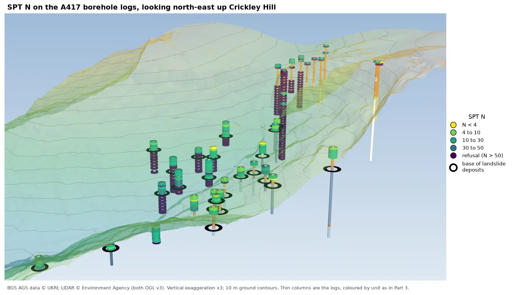
• Part 6: SPT N-values adds the test results, showing which of the printed units are soft and which refuse.
• Multi-colour 3D-printed terrain explains the one-solid-per-colour approach in more detail, including thin colour caps that save filament.
• From DEM to 3D-printable STL starts the 3D-printed maps series from the beginning, with the heightfield solid and the STL writer used here.
• Tiling a large 3D-printed terrain model for a model of the whole A417 route.

Data and licences

• A417 Missing Link ground investigation (BGS deposited data items 173984 and 173975; client Highways England, now National Highways), downloaded through the BGS AGS borehole index and export APIs in Part 5. Contains British Geological Survey materials © UKRI 2026, licensed under the Open Government Licence v3.0.
• Environment Agency LIDAR Composite DTM 1 m, the top surface of the model, from the Defra Data Services Platform WCS. © Environment Agency copyright and/or database right, licensed under the Open Government Licence v3.0. Every figure carries the credit.
• Code: print_ground_model.py, tested with Python 3.12.0, numpy 2.5.4, rasterio 1.5.2, shapely 2.2.0, manifold3d 3.5.5 and pyvista 0.49.2. It runs entirely offline on Part 5’s output.