#Cotswolds

6 posts

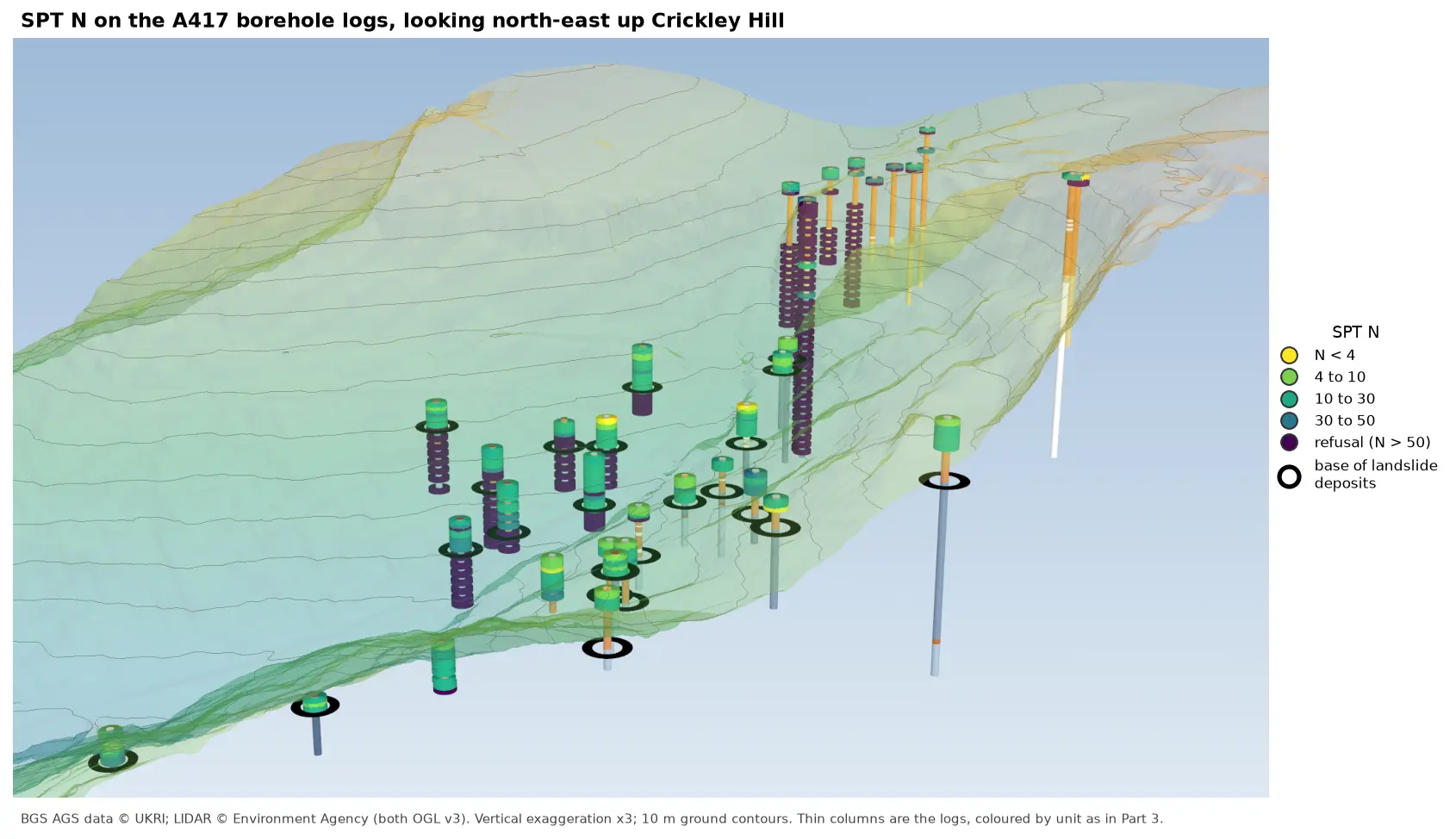
3D view looking north-east up Crickley Hill over semi-transparent LIDAR terrain with 10 m contours. Thin borehole logs coloured by unit carry stacks of coloured discs, one per SPT: yellow and green discs for low N-values near the top of the holes on the escarpment, changing to dark purple refusal discs below black rings that mark the base of the landslide deposits. On the plateau at the top right, the holes turn purple within a few metres of the surface.

Tutorial Python Part 6 of 7

Visualising SPT N-values from AGS4 data in Python

Read the Standard Penetration Tests (ISPT) from a real AGS4 file, separate full tests from refusals, find the stratum each test was made in, and show the N-values four ways: by unit against elevation, across the base of a landslide, as coloured discs on 3D borehole logs over LIDAR terrain, and as a map of the depth to the first refusal.
Intermediate 10 min read

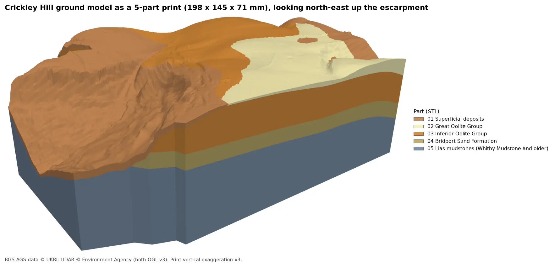
Rendered 3D print of the Crickley Hill ground model, 198 by 145 by 71 mm, looking north-east up the escarpment. Brown superficial deposits cover the western slope, orange Inferior Oolite forms the scarp and plateau, pale yellow Great Oolite caps the south-east, and the side walls show a band of olive Bridport Sand over blue-grey Lias mudstones.

Tutorial Python Part 7 of 7

3D-print a geological ground model: one watertight STL per stratum

Turn the kriged stratum surfaces from Part 5 into a multi-material 3D print of the Cotswold escarpment at Crickley Hill. Cut a window, decide what is too thin to print, build one solid per unit with mesh booleans, prove the parts fit exactly and are watertight, and write five STLs and a colour 3MF for AMS and MMU printers.

Advanced 11 min read

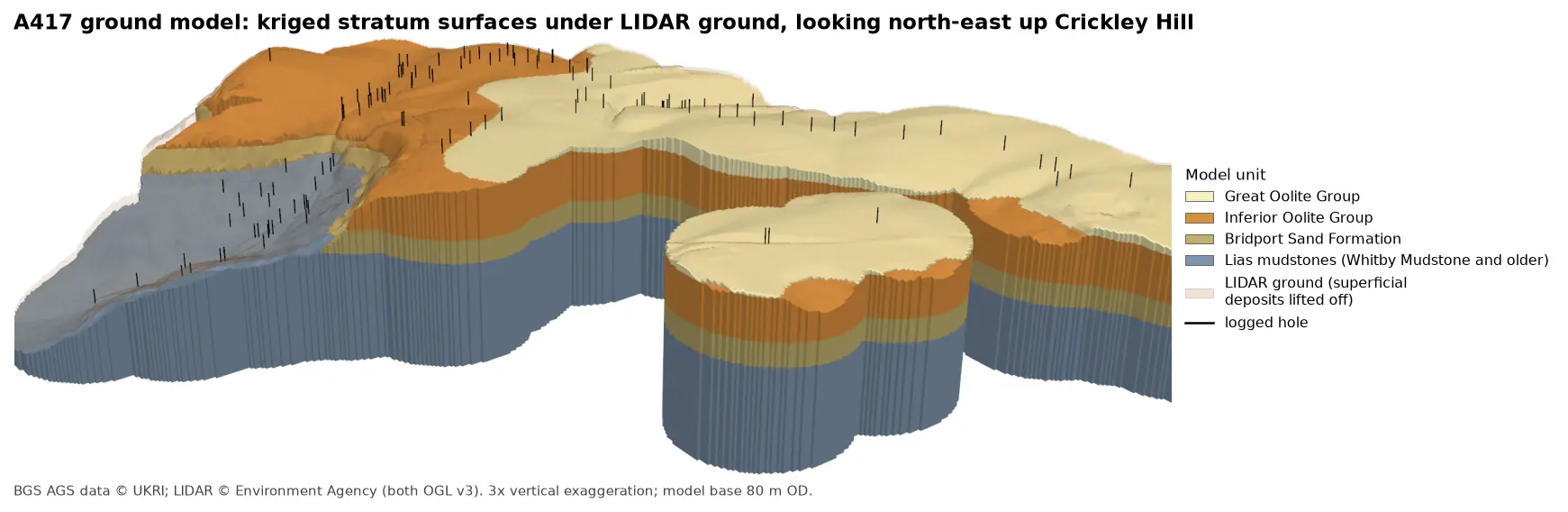
3D block model of the A417 ground model looking north-east up Crickley Hill: blue-grey Lias mudstones form the vale and the lower walls, under a band of olive Bridport Sand, a thick orange band of Inferior Oolite and pale yellow Great Oolite on the plateau. Black vertical lines mark the logged boreholes, and a faint buff skin shows the LIDAR ground lifted off the superficial deposits.

Tutorial Python Part 5 of 7

A 3D ground model from AGS4 boreholes: kriged stratum surfaces in Python

Pick rockhead and the top and base of the key formations from real AGS4 logs, krige them into stratum surfaces under Environment Agency LIDAR ground, and build a 3D ground model of the A417 escarpment in PyVista. Then test it: leave-one-out cross-validation at every borehole, kriging standard deviation maps, a check against every hole that stops short of a surface, and proof that no surface crosses another.

Advanced 15 min read

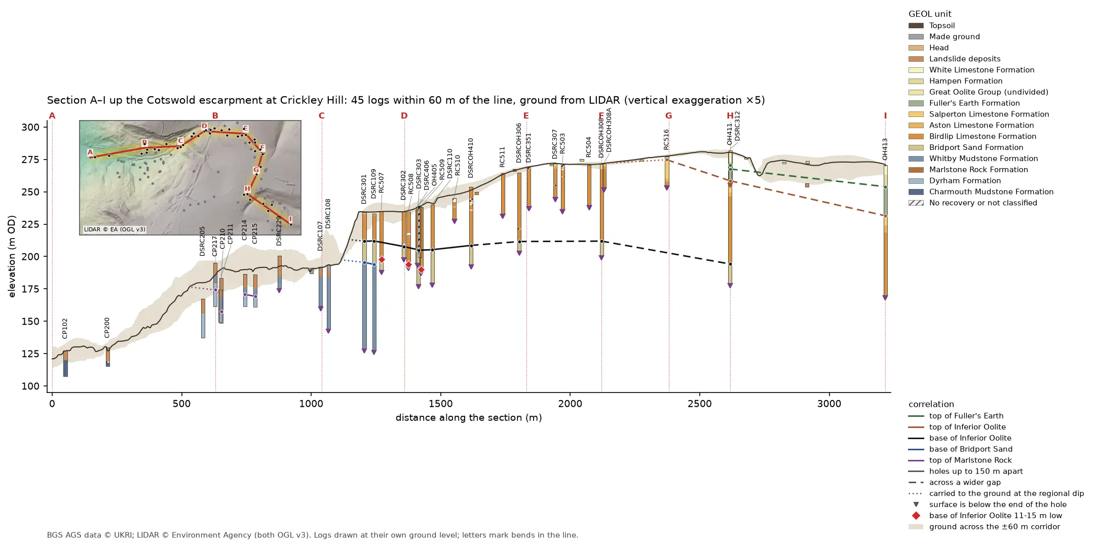
Geological cross-section 3.2 km long from the vale at A, up the Cotswold escarpment at Crickley Hill, to the plateau at I. A dark LIDAR ground line climbs from 121 to 281 m OD over a buff band showing the ground across the corridor. Forty-five strip logs hang below it, coloured by formation: blue-grey Lias mudstone in the vale, orange Inferior Oolite limestone on the escarpment and green Fuller's Earth on the plateau. Coloured lines join the contacts between holes, and red diamonds mark three holes where the base of the limestone is 11 to 15 m low. A map inset at top left shows the bent section line and its corridor on a LIDAR hillshade.

Tutorial Python Part 4 of 7

A geological cross-section from AGS4 boreholes and LIDAR in Python and QGIS

Draw a 3.2 km geological cross-section up the Cotswold escarpment from real AGS4 borehole logs, with the ground profile from Environment Agency LIDAR. Project every hole in a corridor onto the line, pick and correlate the contacts, and measure how much of each correlation line rests on a log and how much is inferred. Then draw the same section with the QGIS elevation profile.

Intermediate 15 min read

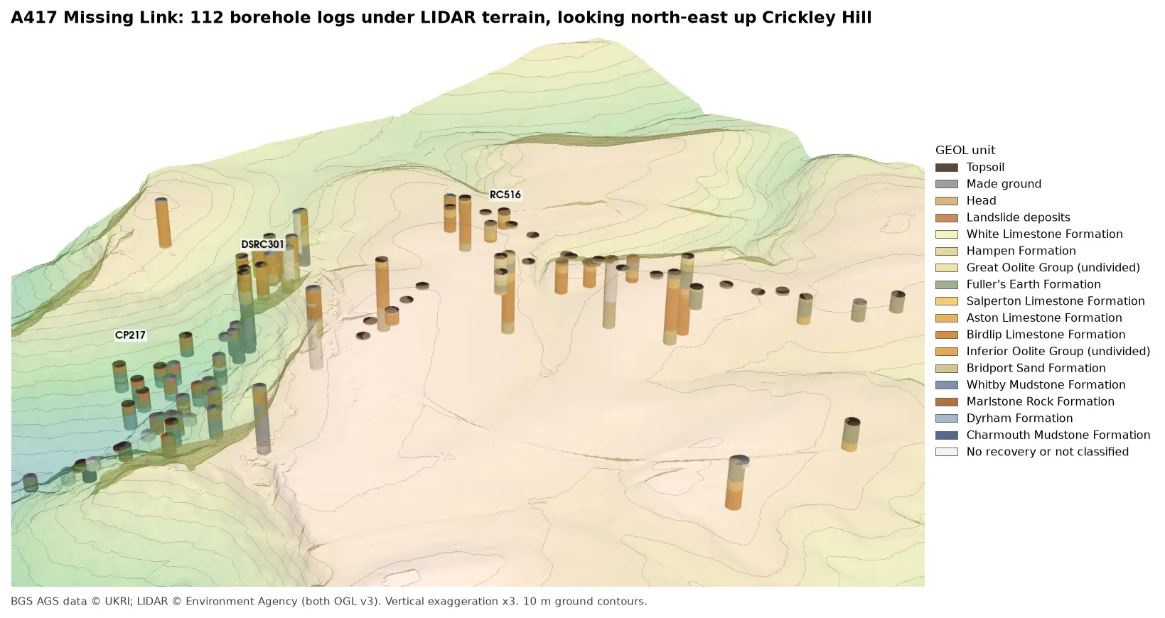
3D view looking north-east up Crickley Hill: LIDAR terrain shaded from green in the vale to buff on the plateau, with 10 m contours, and 112 borehole logs drawn as vertical cylinders coloured by formation. Blue-grey Lias mudstones fill the holes in the vale, orange Inferior Oolite limestones those on the escarpment, and green Fuller's Earth those on the plateau.

Tutorial Python Part 3 of 7

3D borehole logs from AGS4 data in PyVista and QGIS

Build every borehole log in a real AGS4 file as coloured 3D cylinders at their true elevation under Environment Agency LIDAR terrain with PyVista, then style the same intervals in the QGIS 3D map view. Along the way, test whether neighbouring logs agree, and find a block of ground at the top of Crickley Hill where they don't.

Intermediate 12 min read

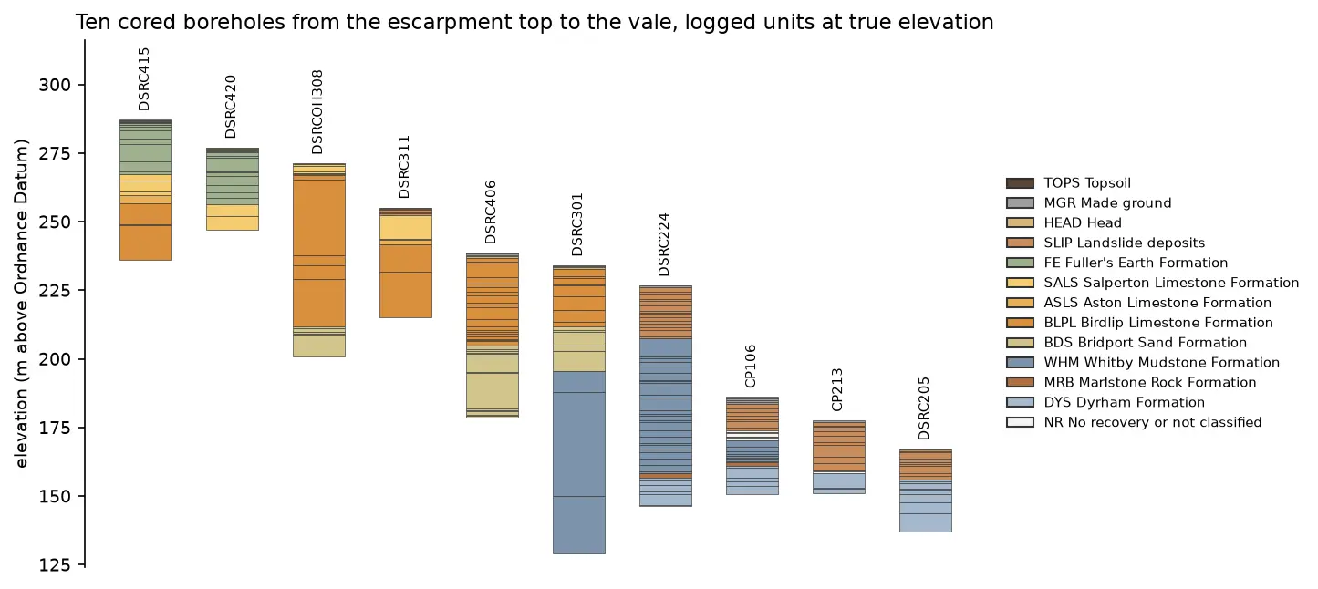
Ten borehole strip logs plotted at true elevation, stepping down from about 287 m above Ordnance Datum on the left to about 167 m on the right. Fuller's Earth and limestone units at the top give way to Bridport Sand, then thick blue-grey Whitby Mudstone and Dyrham Formation in the lower holes.

Tutorial Python Part 1 of 7

Read and validate AGS4 ground investigation data with Python

Find a real ground investigation in the British Geological Survey's AGS archive, download it as AGS4, learn how the file is put together, read it into pandas with python-ags4, fix every error the AGS checker reports, and check that the borehole logs make geological sense. The example is the A417 Missing Link at Crickley Hill.

Intermediate 12 min read