Read and validate AGS4 ground investigation data with Python
Find a real ground investigation in the British Geological Survey's AGS archive, download it as AGS4, learn how the file is put together, read it into pandas with python-ags4, fix every error the AGS checker reports, and check that the borehole logs make geological sense. The example is the A417 Missing Link at Crickley Hill.
- Level
- Intermediate
- Tested with
- Python 3.12
- Source code
- Download scripts
Key takeaways
- An AGS4 file is a set of tables. Each GROUP has HEADING, UNIT and TYPE rows and then DATA rows, and python-ags4 reads each group into a pandas DataFrame.
- The BGS archive exported the A417 Missing Link's 112 holes as three files that drew 8,866 checker messages between them. Ten small, explained fixes brought that to zero rule errors.
- A file can pass the checker and still hold surprises. A stratigraphic order test found one borehole, CP217, with the Lias sequence repeated beneath landslide deposits.
Before you start
- Python 3.10+ with python-ags4, pandas, numpy, requests and matplotlib
- Basic pandas: filtering rows, groupby and value_counts
- No geotechnical background is assumed; the AGS groups are explained as they come up
Almost every ground investigation in the UK hands over its borehole data as an AGS file, and most GIS people meet one sooner or later. This series takes a real one from start to finish: reading it, putting it on a map, building it in 3D, and on to cross-sections and ground models. In this first part we find the data, open it up, validate it, fix what the checker finds, and then check something the checker can’t: whether the logs make geological sense.
Our example is the A417 Missing Link, the scheme to replace the single-carriageway stretch of the A417 between Brockworth and Cowley, where the road climbs the Cotswold escarpment at Crickley Hill in Gloucestershire. Its ground investigation is a good teacher. It has 112 exploratory holes, some over 100 m deep, through Jurassic limestones, sands and mudstones, on a hillside with mapped landslides. The British Geological Survey (BGS) holds the data, and you can download it under the Open Government Licence.
We use python-ags4, the open-source library maintained by the AGS’s own data format working group. The steps are:
- find the boreholes in the BGS AGS index;
- download them as AGS4 files;
- look at how an AGS4 file is built;
- read every group into pandas;
- explore LOCA, GEOL and SAMP, the three groups GIS work leans on most;
- validate the files with the AGS checker;
- fix every error and write a clean file;
- check the geology.
The full script is read_validate_ags4.py, with a small helper module, a417_ags.py, that later parts reuse.
Step 1: find the boreholes in the BGS index
The BGS keeps AGS data donated by the ground investigation industry, and publishes an index of every borehole it can export through its OGC API. Each submission is a numbered deposited data item; the A417 Missing Link ground investigation is item 173984. One request returns every hole in it as GeoJSON:
ITEM = 173984                       # BGS deposited data item: HE551505 A417 Missing Link GIINDEX = "https://ogcapi.bgs.ac.uk/collections/agsboreholeindex/items"
def borehole_index(item=ITEM): """Every borehole in one BGS deposited data item, from the BGS OGC API (GeoJSON).""" r = requests.get(INDEX, params={"f": "json", "limit": 1000, "item_index_id": item}, headers=UA, timeout=120) r.raise_for_status() rows = [f["properties"] for f in r.json()["features"]] return pd.DataFrame(rows).sort_values("bgs_loca_id").reset_index(drop=True)=== Step 1: the A417 Missing Link in the BGS AGS borehole index ===HE551505 A417 MISSING LINK GROUND INVESTIGATION112 exploratory holes | deepest 105.0 m | E 392,081 to 394,938 | N 213,164 to 216,419 bgs_loca_id loca_id x y loca_fdep2026081011400291004 CP102 392080.9 215724.9 20.002026081011400291005 CP104 392524.7 215642.0 15.002026081011400291006 CP104A 392525.2 215641.5 16.76The coordinates are British National Grid eastings and northings, which Part 2 puts on a map.
Step 2: download as AGS4
The BGS AGS export API returns a ZIP containing an AGS4 file for the boreholes you list. A URL can only hold so many IDs, so we ask for 40 at a time, keep the files, and never download twice:
EXPORT = "https://agsapi.bgs.ac.uk/v7/ags_export/"BATCH = 40
def download(data_dir, item=ITEM): raw = Path(data_dir) / f"bgs_{item}" raw.mkdir(parents=True, exist_ok=True) if not list(raw.glob("*.ags")): ids = borehole_index(item).bgs_loca_id.tolist() for i in range(0, len(ids), BATCH): r = _get(EXPORT, {"bgs_loca_id": ";".join(ids[i:i + BATCH])}) with zipfile.ZipFile(io.BytesIO(r.content)) as z: for name in z.namelist(): (raw / f"batch{i // BATCH + 1:02d}_{Path(name).name}").write_bytes(z.read(name)) time.sleep(1) return sorted(raw.glob("*.ags"))=== Step 2: download as AGS4, 40 holes per request ===batch01_202608101140029.ags: 476 kB, 3,958 linesbatch02_202608101140029.ags: 493 kB, 3,806 linesbatch03_202608101140029.ags: 112 kB, 1,102 linesStep 3: what an AGS4 file looks like
Open an AGS4 file in a text editor and you will see something like a stack of CSV tables. Each table, called a group, starts with a GROUP line and then three header rows before its data:
=== Step 3: what an AGS4 file looks like ==="GROUP","LOCA""HEADING","LOCA_ID","LOCA_TYPE","LOCA_STAT","LOCA_NATE","LOCA_NATN","LOCA_GREF","LOCA_GL","LOCA_ ..."UNIT","","","","m","m","","m","","m","yyyy-mm-dd","","","yyyy-mm-dd","","m","m","m","","","m"," ..."TYPE","ID","PA","PA","U","U","X","U","X","U","DT","X","X","DT","X","X","X","X","X","X","X","X", ..."DATA","CP102","RC","FINAL","392080.9","215724.9","","127.55","","20","","","","","","","","","" ..."DATA","CP104","CP","FINAL","392524.7","215642","","148","Borehole terminated at 15.00m followin ...- HEADING names the columns. Every heading starts with its group name, so
LOCA_NATEis the National Grid easting in the LOCA group. - UNIT gives the units, here metres for the coordinates, ground level (
LOCA_GL) and final depth (LOCA_FDEP). - TYPE says how to read each value:
IDfor a key,PAfor a code explained in the ABBR group,Xfor free text,DTfor a date, andUfor a number written to however many decimal places the data deserves. - DATA rows hold the values, one row per record.
Groups are linked by key fields. LOCA_ID names an exploratory hole in LOCA, and every geology layer, sample and test belonging to that hole repeats the same LOCA_ID. That is what makes AGS so easy to join in pandas or a GIS.
Step 4: read every group into pandas
AGS4.AGS4_to_dataframe() returns two dictionaries keyed by group name: one of DataFrames and one of heading lists. The UNIT and TYPE rows stay at the top of each DataFrame, which keeps a round trip back to AGS lossless:
tables, headings = AGS4.AGS4_to_dataframe(str(paths[0]))print(f"{len(tables)} groups in {paths[0].name}: {' '.join(tables)}")print(tables["LOCA"][["HEADING", "LOCA_ID", "LOCA_TYPE", "LOCA_NATE", "LOCA_NATN", "LOCA_GL"]].head(4) .to_string(index=False))16 groups in batch01_202608101140029.ags: PROJ UNIT TYPE TRAN FILE DICT ABBR LOCA GEOL BKFL CDIA PIPE WSTG WSTD ISPT SAMPHEADING LOCA_ID LOCA_TYPE LOCA_NATE LOCA_NATN LOCA_GL UNIT m m m TYPE ID PA U U U DATA CP102 RC 392080.9 215724.9 127.55 DATA CP104 CP 392524.7 215642 148The three downloads are one project, so merge() in a417_ags.py stacks them group by group. It keeps the UNIT and TYPE rows once, and drops rows that every file repeats, such as the project details in PROJ and the abbreviations in ABBR:
def merge(paths): tables, headings = {}, {} for p in paths: t, h = AGS4.AGS4_to_dataframe(str(p)) for group, df in t.items(): if group not in tables: tables[group], headings[group] = df, list(h[group]) continue headings[group] += [c for c in h[group] if c not in headings[group]] tables[group] = pd.concat([tables[group], df[df.HEADING == "DATA"]], ignore_index=True) for group, df in tables.items(): df = df.reindex(columns=headings[group]).fillna("") tables[group] = df.drop_duplicates(ignore_index=True) return tables, headingspython-ags4 ships the standard AGS4 data dictionary, so we can label each group with its official description:
All three files stacked, DATA rows per group: SAMP 4,555 Sample Information GEOL 1,564 Field Geological Descriptions ISPT 415 Standard Penetration Test Results BKFL 354 Exploratory Hole Backfill Details PIPE 136 Monitoring Installation Pipe Work CDIA 127 Casing Diameter by Depth LOCA 112 Location Details WSTG 24 Water Strike - General WSTD 23 Water Strike - Details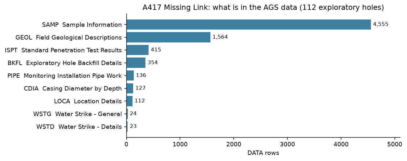
This export has no laboratory results and no groundwater monitoring readings (MONG). That matters later in the series, and it is the first thing worth checking in any AGS file you are given.
Step 5: LOCA, GEOL and SAMP
Three groups do most of the work in GIS:
- LOCA, one row per exploratory hole: its type, coordinates, ground level and final depth.
- GEOL, one row per layer in the log: its top and base depths, the logger’s description, and codes for the geological unit.
- SAMP, one row per sample taken: its depth, type and reference, so laboratory results can be traced back to a place in the ground.
python-ags4 reads everything as text. AGS4.convert_to_numeric() turns columns into numbers using the TYPE row, but it leaves U columns as text, so numeric() in the helper converts those too and keeps only the DATA rows:
def numeric(tables): out = {} for g, df in tables.items(): types = df[df.HEADING == "TYPE"].iloc[0] n = AGS4.convert_to_numeric(df) for col in types.index[types == "U"]: n[col] = pd.to_numeric(n[col], errors="coerce") out[g] = n return out=== Step 5: LOCA, GEOL and SAMP ===LOCA_TYPE: {'RC': 71, 'TP': 30, 'CPT': 6, 'RO': 3, 'CP': 2}LOCA_CLST: {'PHASE 2A.1': 99, 'PHASE 1': 8, 'PHASE 2A': 5}ground level 127.5 to 294.1 m OD | final depth 0.8 to 105.0 m
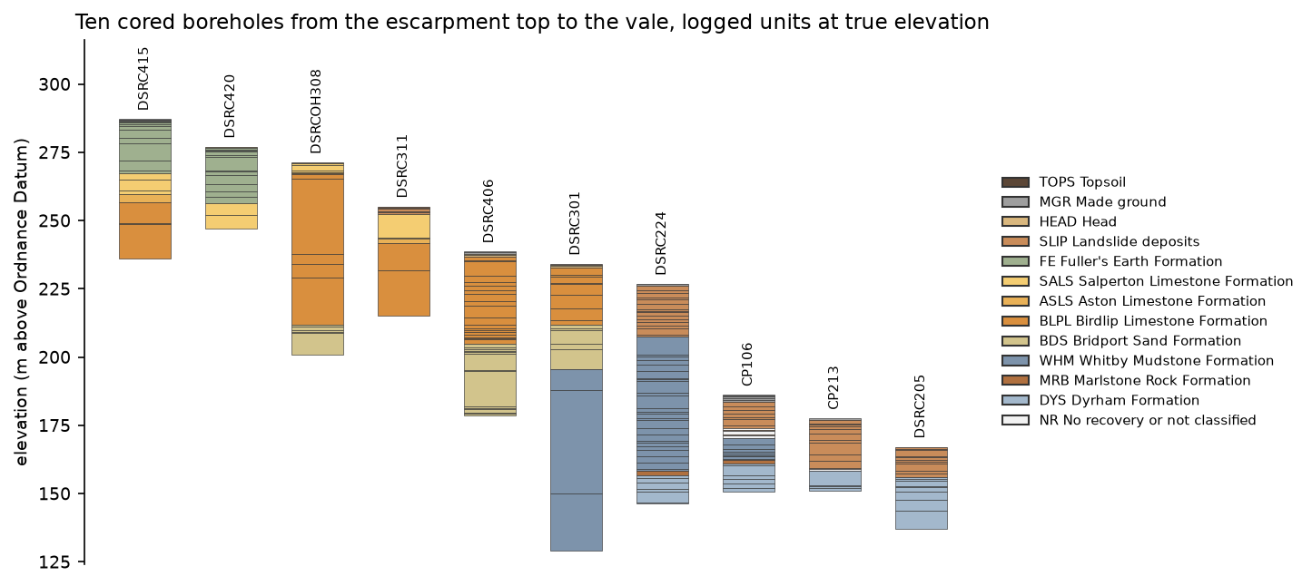
GEOL: 1,564 strata in 112 holes. One borehole, top to bottom: GEOL_TOP GEOL_BASE GEOL_GEOL GEOL_BGS GEOL_DESC 0.00 0.20 TOP Grass over soft dark brown gravelly silty CLAY ... 0.20 0.75 HDD HEAD Soft to firm orangish brown slightly gravelly C... 0.75 1.20 HDD HEAD Firm orange and light grey slightly sandy sligh... 1.20 2.60 FEF FE Stiff bluish grey mottled orangish brown and re... 2.60 2.70 IOG SALS Limited recovery. Single angular irregular lime... 2.70 3.30 No recovery. 3.30 4.40 IOG SALS Weak to medium strong bioclastic LIMESTONE with... ... 17.35 19.60 IOG ASLS Weak light grey and light brown bioclastic LIME... 19.60 22.20 IOG BLPL Weak light brown bioclastic and ooidal LIMESTON...
SAMP: 4,555 samples. SAMP_TYPE: {'C': 1855, 'CS': 838, 'D': 830, 'ES': 370, 'B': 326, 'L': 205, 'EW': 78, 'UT': 26} C = Core sample | CS = Core sample (prepared) | D = Small disturbed sample | ES = Soil sample for environmental testing | B = Bulk disturbed sample | L = Liner sample (dynamic) | EW = Water sample for environmental testing | UT = Thin wall open drive tube samplerMost of the holes are rotary cored boreholes (RC) and trial pits (TP). The borehole above, RC516, shows the two unit codes side by side. GEOL_GEOL is the project’s own code (IOG for Inferior Oolite Group), and GEOL_BGS is the code from the BGS Lexicon of Named Rock Units, which here splits the Inferior Oolite into its Salperton, Aston and Birdlip Limestone formations. We use the Lexicon code wherever there is one.
Step 6: validate with the AGS checker
AGS4.check_file() tests a file against the AGS4 rules and returns a dictionary of problems keyed by rule. Here is the count for each download:
def error_counts(path): errors = AGS4.check_file(str(path)) return {rule: len(v) for rule, v in errors.items() if rule not in ("Metadata", "Summary of data", "General")}=== Step 6: validate the downloads with the AGS checker === batch01_202608101140029.ags batch02_202608101140029.ags batch03_202608101140029.ags totalAGS Format Rule 2a 3958 3806 1102 8866AGS Format Rule 19a 8 8 5 21AGS Format Rule 19b 6 6 6 18AGS Format Rule 1 1 3 0 4AGS Format Rule 20 2 2 2 6AGS Format Rule 7 5 5 4 14AGS Format Rule 9 8 8 5 21AGS Format Rule 10a 6 6 6 18AGS Format Rule 10c 6 6 4 16FYI (Related to Rule 16) 8 8 8 24AGS Format Rule 1: Has Non-ASCII character(s) (assuming that file encoding is 'utf-8'). (line 1146)AGS Format Rule 9: BGS_PROJ_ID not found in DICT group or the standard AGS4 dictionary. (line 2)AGS Format Rule 10a: Duplicate key field combination: DATA|HEADING|LOCA|LOCA_ORID (line 99)AGS Format Rule 10c: Parent entry for line not found in LOCA: X (line 1301)Don’t be put off by the numbers. Nearly all of them are the same few problems repeated, and none of them means the measurements are wrong:
| Rule | What the checker found | Cause |
|---|---|---|
| 2a | every line | lines end in LF; AGS4 needs CR+LF |
| 1 | 4 lines | a degree sign double-encoded as Β° |
| 19a, 19b | BGS_PROJ_ID, BGS_LOCA_ID | longer than 9 characters, and not prefixed by their group name |
| 9 | the same headings | not in the standard dictionary and not defined in DICT |
| 7 | heading order | headings must follow the dictionary’s order |
| 10a | DICT | three user-defined headings defined twice |
| 10c | every child group | LOCA_ID exported with TYPE X instead of ID, so it no longer matches its parent |
| 20 | FILE | the file refers to a FILE folder that isn’t there |
| 16 (FYI) | ABBR | two abbreviation descriptions differ from the standard list’s wording |
Step 7: merge, repair and write a clean file
repair() in a417_ags.py fixes each of these in turn, with a comment for each rule. Two of the fixes are worth showing in full. The first renames the BGS identifiers to valid AGS headings and defines them in DICT:
for group, old, new, desc in [("PROJ", "BGS_PROJ_ID", "PROJ_BGSI", "BGS export project identifier"), ("LOCA", "BGS_LOCA_ID", "LOCA_BGSI", "BGS borehole index identifier")]: tables[group] = tables[group].rename(columns={old: new}) tables[group].loc[tables[group].HEADING == "TYPE", new] = "X" headings[group] = [new if c == old else c for c in headings[group]] new_dict.append({"HEADING": "DATA", "DICT_TYPE": "HEADING", "DICT_GRP": group, "DICT_HDNG": new, "DICT_STAT": "OTHER", "DICT_DTYP": "X", "DICT_DESC": desc})The second restores the key type that links every child group to LOCA:
for group, df in tables.items(): if group != "LOCA" and "LOCA_ID" in df: df.loc[df.HEADING == "TYPE", "LOCA_ID"] = "ID"There was one more thing to find, which the checker doesn’t report. The export adds a _TEXT twin to depth columns, such as GEOL_TOP_TEXT next to GEOL_TOP. The twins hold the values as the logger wrote them (0.50), while the plain columns have been reformatted (0.5). repair() asserts that each pair agrees as numbers, puts the original text back and drops the twin, so no precision is lost.
AGS4.dataframe_to_AGS4() writes the result with CR+LF line endings, and write() adds the FILE folder that Rule 20 expects. Then we check each stage again:
=== Step 7: merge, repair and write a clean file ===double-encoded degree signs to repair: 4wrote output/clean/A417_missing_link_GI.ags (1,031 kB) with FILE/BGSFileSet01 beside itCRLF line endings: True downloads merged and rewritten repairedAGS Format Rule 2a 8866 0 0FYI (Related to Rule 16) 24 8 8AGS Format Rule 19a 21 8 0AGS Format Rule 9 21 8 0AGS Format Rule 19b 18 6 0AGS Format Rule 10a 18 6 0AGS Format Rule 10c 16 6 0AGS Format Rule 7 14 5 0AGS Format Rule 20 6 0 0AGS Format Rule 1 4 4 0left in the clean file: no rule errors FYI: HDPH_TYPE: Description of abbreviation "IP" is "Hand dug inspection pit" but it should be "Inspection pit" according to the standard abbreviations list. FYI: HDPH_TYPE: Description of abbreviation "WLS" is "Windowless sampler" but it should be "Dynamic (windowless) sampler" according to the standard abbreviations list.clean file reads back identically: True | load_clean() groups: 16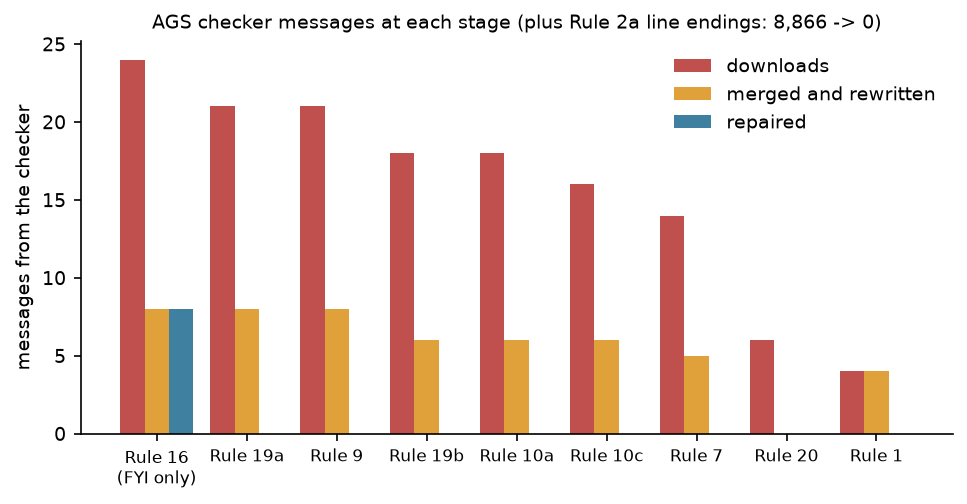
The remaining FYI notes say that the project described two abbreviations in its own words. That isn’t an error. The project’s wording is part of the record, so we leave it as it is.
Step 8: check the logs make geological sense
A file that passes every rule can still describe impossible ground. The checker knows nothing about geology, so we test the logs ourselves. The helper has a table of the units met here, youngest first, each with a rank giving its expected place in the sequence. unit_code() gives every GEOL layer one of these codes, using the BGS Lexicon code where there is one and the project’s code otherwise. Here is how many layers each unit covers:
=== Step 8: check the logs make geological sense ===Units, youngest first:codeTOPS Topsoil 66MGR Made ground 85HEAD Head 54SLIP Landslide deposits 320WHL White Limestone Formation 11HMB Hampen Formation 21GOG Great Oolite Group (undivided) 7FE Fuller's Earth Formation 156SALS Salperton Limestone Formation 63ASLS Aston Limestone Formation 25BLPL Birdlip Limestone Formation 322IOG Inferior Oolite Group (undivided) 1BDS Bridport Sand Formation 101WHM Whitby Mudstone Formation 125MRB Marlstone Rock Formation 12DYS Dyrham Formation 109CHAM Charmouth Mudstone Formation 20NR No recovery or not classified 66For every hole the script then checks that each layer’s base is below its top, that the layers meet with no gaps or overlaps, that nothing is logged below the final depth, that superficial deposits don’t appear beneath bedrock, and that the bedrock never steps back up to a younger unit:
def in_order(codes): """True if a top-to-bottom list of bedrock unit codes never steps back to a younger unit.""" reached = 0 for code in codes: if UNITS.at[code, "last"] < reached: return False reached = max(reached, UNITS.at[code, "rank"]) return True112 holes with GEOL, 90 reach bedrock. Holes needing a second look: CP217: bedrock out of order: WHM > MRB > DYS > WHM > MRB > DYS CPT202: gap or overlap of -0.40 mOf 1,564 layers in 112 holes, only two holes need a second look. CPT202 has a 0.40 m overlap between two layers, a small slip in the log. CP217 is more interesting.
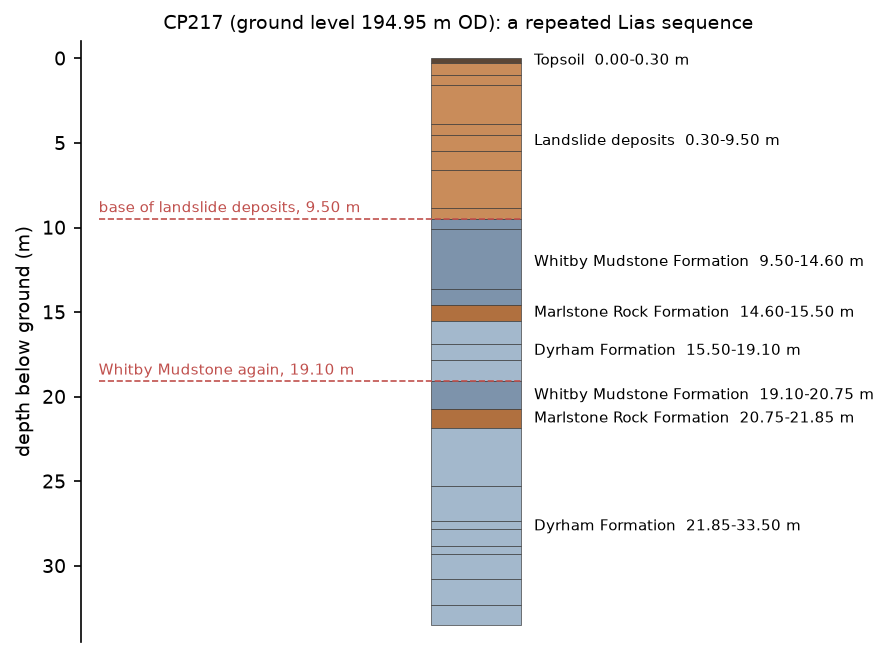
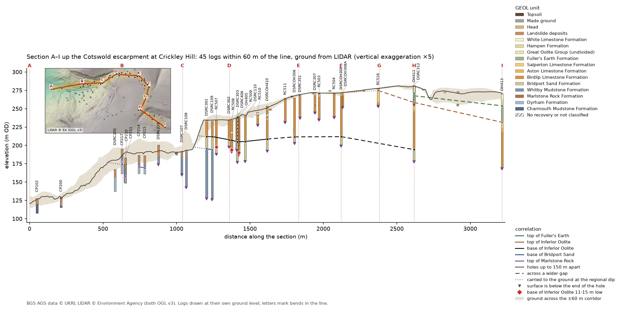
CP217 is near the foot of the escarpment, where the BGS maps landslides. Below 9.2 m of landslide deposits it logs Whitby Mudstone, Marlstone Rock and Dyrham Formation, and then, from 19.10 m, the same three units again. The two Marlstone Rock beds are 6.15 m apart vertically and are described in much the same way: medium strong grey limestone. On a landslipped slope, the most likely explanation is that the upper sequence is a block of Lias that slid down the slope more or less intact and now rests on the sequence still in place. A fault repeating the beds would give the same log, so the next step is to compare CP217 with its neighbours. Part 3 puts every log side by side in 3D, and the cross-sections in Part 4 are the natural way to test it.
Frequently asked questions
What is an AGS file?
A plain-text file in the Association of Geotechnical and Geoenvironmental Specialists’ data format, used to exchange ground investigation data in the UK and elsewhere. It holds a set of tables, called groups, for locations, geology, samples, in-situ tests, laboratory results and monitoring, linked by key fields such as LOCA_ID.
How do I open an AGS file in Python?
Install python-ags4 and call AGS4.AGS4_to_dataframe("file.ags"). It returns a dictionary of pandas DataFrames, one per group, and a dictionary of their headings. Use AGS4.convert_to_numeric() before doing arithmetic, because every value is read as text.
How do I check an AGS file for errors?
Call AGS4.check_file("file.ags"), or use the ags4_cli check command that comes with python-ags4. Both test the file against the AGS4 rules and report each problem with its rule number and line. The AGS also runs an online validator.
Where can I download AGS data for free?
The British Geological Survey holds AGS submissions donated by the industry. Find them on the GeoIndex map or through the BGS OGC API borehole index, and export them through the BGS AGS API. Much of it is available under the Open Government Licence; check the licence of each submission.
Can I load an AGS file straight into QGIS or ArcGIS?
Not directly. Read it with python-ags4, join the groups you need on LOCA_ID, and make points from LOCA_NATE and LOCA_NATN. Part 2 of this series does exactly that and writes a GeoPackage that both programs open.
Next steps
- Part 2: Boreholes on a map turns LOCA into points in British National Grid, checks every ground level against LIDAR and builds a QGIS project with labels and popups.
- Part 3: 3D borehole logs builds every log in 3D with PyVista and QGIS and tests whether neighbouring logs agree.
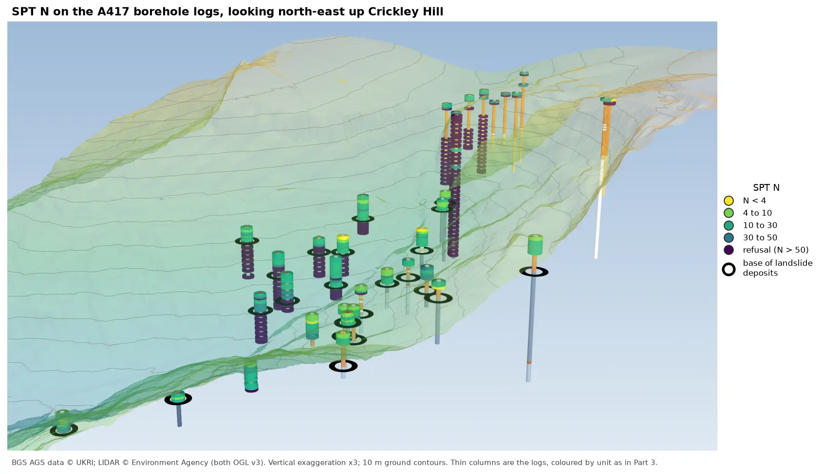
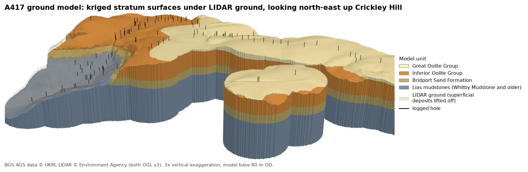
- Later in the series: cross-sections along a line of boreholes with LIDAR ground level, interpolated stratum surfaces, test results such as SPT N-values, and a 3D-printed ground model.
- New to coordinates? Coordinate reference systems in Python explains why British National Grid matters for Part 2.
Data and licences
- A417 Missing Link ground investigation (BGS deposited data item 173984; client Highways England, now National Highways; contractor Geotechnical Engineering Ltd), downloaded through the BGS AGS borehole index and export APIs. Contains British Geological Survey materials © UKRI 2026, licensed under the Open Government Licence v3.0.
- Code:
read_validate_ags4.pyanda417_ags.py, tested with Python 3.12.0, python-ags4 1.2.0, pandas 2.3.3, numpy 2.5.4 and matplotlib 3.11.2. The only network requests are to the BGS index and export APIs; everything else runs locally.
Key terms
- AGS4
- The Association of Geotechnical and Geoenvironmental Specialists' data transfer format, version 4: a plain-text, comma-separated file of tables (groups) used across the UK ground investigation industry.
- Group
- One table in an AGS file, such as LOCA (locations), GEOL (geology descriptions) or SAMP (samples). Its rows are linked to other groups by key fields such as LOCA_ID.
- Exploratory hole
- Any point investigation in the ground: a borehole, trial pit, cone penetration test or window sample. AGS stores them all in LOCA.
- Rockhead
- The top of bedrock beneath soil, made ground and other superficial deposits.
- m OD
- Metres above Ordnance Datum, the mean sea level reference (Newlyn) used for heights in Great Britain.
Data for this tutorial
- BGS AGS borehole data · Donated AGS ground investigation data, Open Government Licence
Licences and formats for each source are listed in the GIS data sources catalogue.