Boreholes on a map: AGS4 locations in British National Grid with QGIS
Turn the LOCA group of a real AGS4 file into points in British National Grid, see what happens when the CRS is wrong, summarise each hole's geology from GEOL, check every ground level against Environment Agency LIDAR, and build a QGIS project with labels and a map tip that shows the borehole log.
- Level
- Intermediate
- Tested with
- Python 3.12
- Source code
- Download scripts
Key takeaways
- LOCA_NATE and LOCA_NATN are British National Grid metres, so the points belong in EPSG:27700. Swapping them, or calling them longitude and latitude, puts boreholes in the sea or nowhere at all.
- Joining a summary of GEOL to LOCA gives every point its depth to rock and the formation at rockhead: 90 of the 112 A417 holes reach bedrock, at a median depth of 1.20 m.
- Comparing LOCA_GL with Environment Agency LIDAR is a quick check on any AGS file. Here 103 of 112 ground levels agree within 0.5 m, and the three that differ by more than 1 m are worth a look.
- A QGIS map tip can show the whole borehole log when you hover over a point, from one HTML field written by Python.
Before you start
- Part 1 of this series, or at least its helper module a417_ags.py
- Python 3.10+ with python-ags4, GeoPandas, rasterio, pyproj, requests and matplotlib
- QGIS 3.34 or later for the QGIS project (tested with 3.40 LTR)
An AGS file knows exactly where every borehole is, but it doesn’t draw a map. In Part 1 we read, validated and repaired the ground investigation for the A417 Missing Link at Crickley Hill in Gloucestershire. Now we put its 112 exploratory holes on a map, check their ground levels against the Environment Agency’s LIDAR, and build a QGIS project where hovering over any hole shows its log.
The steps are:
- turn LOCA into points in British National Grid;
- see what goes wrong with the wrong CRS;
- summarise GEOL for each hole;
- check every ground level against LIDAR;
- draw the maps;
- write a GeoPackage and style it in QGIS with PyQGIS.
The code is boreholes_map.py for Steps 1 to 6 and qgis_borehole_map.py for the QGIS project. Both use a417_ags.py from Part 1, which downloads the data on the first run.
Step 1: LOCA to points in British National Grid
In UK investigations, LOCA_NATE and LOCA_NATN are British National Grid eastings and northings in metres. The CRS to give them is EPSG:27700. With GeoPandas that is one line:
ags = A.load_clean(DATA)loca = ags["LOCA"]holes = gpd.GeoDataFrame(loca, geometry=gpd.points_from_xy(loca.LOCA_NATE, loca.LOCA_NATN), crs="EPSG:27700")=== Step 1: LOCA to points in British National Grid ===112 holes | CRS OSGB36 / British National Grid (EPSG:27700)extent E 392,081 to 394,938, N 213,164 to 216,419centre in WGS84: 51.83674 N, 2.09630 W (Crickley Hill and Birdlip)Converting the centre to latitude and longitude is a quick sanity check: 51.84° N, 2.10° W is on the Cotswold edge between Cheltenham and Gloucester, exactly where the A417 climbs Crickley Hill.
Step 2: what goes wrong with the wrong CRS
Two mistakes catch people out. The first is swapping easting and northing, easily done when a spreadsheet’s columns are labelled X and Y. The second is tagging the points as longitude and latitude (EPSG:4326), which some tools do by default when they see two numeric columns:
to_wgs = Transformer.from_crs("EPSG:27700", "EPSG:4326", always_xy=True)lon, lat = to_wgs.transform(first.LOCA_NATN, first.LOCA_NATE) # easting and northing swappedwrong = gpd.GeoDataFrame(geometry=gpd.points_from_xy(loca.LOCA_NATE, loca.LOCA_NATN), crs="EPSG:4326")=== Step 2: what goes wrong with the wrong CRS ===CP102 with easting and northing swapped lands at 53.393 N, -4.773 W: in the sea off north Wales, 249 km awaytagged as EPSG:4326 instead, x runs to 394,938 'degrees'; valid longitudes stop at 180, so nothing can be drawnIf your boreholes turn up in the Irish Sea or refuse to appear at all, these are the first two things to check. Coordinate reference systems in Python goes into CRSs in more depth.
Step 3: summarise GEOL for each hole
A point is only as useful as its attributes. GEOL has one row per layer, so we summarise it to one row per hole and join that to the points. UNIT comes from Part 1’s load_clean(), and the unit table’s rank tells bedrock (rank above 0) from topsoil, made ground, head and landslide deposits (rank 0):
geol = ags["GEOL"].copy()geol["rank"] = geol.UNIT.map(A.UNITS["rank"])rock = geol[geol["rank"] > 0].groupby("LOCA_ID")summary = pd.DataFrame({ "rockhead_depth": rock.GEOL_TOP.min(), "rockhead_unit": rock.UNIT.first(), "deepest_unit": rock.UNIT.last(),})water = ags["WSTG"].groupby("LOCA_ID").WSTG_DPTH.min().rename("first_water_strike")We also count each hole’s samples (SAMP) and Standard Penetration Tests (ISPT), take the description of each LOCA_TYPE code from the ABBR group, and build a small HTML table of the log for the QGIS map tip in Step 6:
def log_html(g): """The hole's log as a small HTML table, one row per unit, for the QGIS popup.""" runs = g.groupby((g.UNIT != g.UNIT.shift()).cumsum()).agg( unit=("UNIT", "first"), top=("GEOL_TOP", "min"), base=("GEOL_BASE", "max")) rows = "".join(f'<tr><td style="background:{A.UNITS.colour[r.unit]};width:10px"></td>' f"<td>{r.top:.2f}–{r.base:.2f} m</td><td>{escape(A.UNITS.name[r.unit])}</td></tr>" for r in runs.itertuples()) return f'<table style="font-size:11px;border-collapse:collapse">{rows}</table>'The groupby on (g.UNIT != g.UNIT.shift()).cumsum() merges consecutive layers of the same unit, so a run of separately described Birdlip Limestone layers becomes one row.
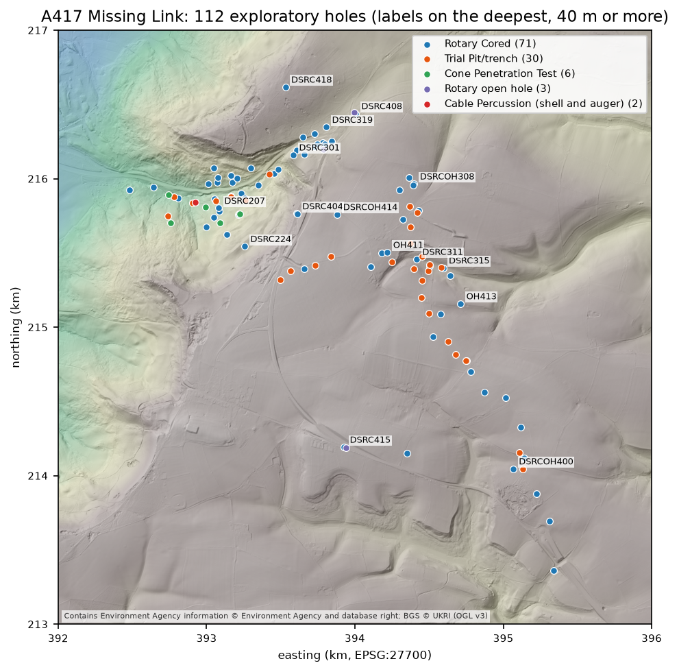
=== Step 3: summarise GEOL for each hole ===type_nameRotary Cored                          71Trial Pit/trench                      30Cone Penetration Test                  6Rotary open hole                       3Cable Percussion (shell and auger)     2
90 holes reach bedrock; depth to rock 0.10 to 20.70 m (median 1.20 m)unit at rockhead: {'FE': 20, 'BLPL': 17, 'WHM': 15, 'SALS': 9, 'ASLS': 5, 'GOG': 5, 'DYS': 5, 'HMB': 5, 'WHL': 4, 'CHAM': 3, 'MRB': 1, 'IOG': 1}LOCA_ID    type_name  LOCA_GL  LOCA_FDEP  rockhead_depth  rockhead_mOD             rockhead_name first_water_strike  n_samples  CP217 Rotary Cored   194.95       33.5            9.50        185.45 Whitby Mudstone Formation               2.25         61DSRC415 Rotary Cored   287.20       51.0            0.75        286.45  Fuller's Earth Formation                NaN         53  RC516 Rotary Cored   277.35       22.2            1.20        276.15  Fuller's Earth Formation                NaN         35
On the plateau, bedrock is close to the surface: DSRC415 and RC516 reach the Fuller’s Earth Formation within 1.2 m. Down the escarpment, CP217 goes through 9.2 m of landslide deposits first. Fifteen of the 22 holes that never reach bedrock are trial pits and cone penetration tests, which stop in the soils and superficial deposits.
Step 4: check every ground level against LIDAR
LOCA_GL is the ground level at each hole, normally surveyed when the hole was set out. The Environment Agency’s LIDAR composite DTM gives an independent ground level for almost all of England, so comparing the two is a quick check on the survey and on the coordinates: a hole in the wrong place often shows up as a ground level that doesn’t match.
The script asks the Defra Web Coverage Service (WCS) for a 4 × 4 km DTM at 2 m resolution in 1 km tiles, caches the tiles in data/, and mosaics them. It then reads the DTM at each hole:
col = ((holes.LOCA_NATE - X0) / RES).astype(int)row = ((Y1 - holes.LOCA_NATN) / RES).astype(int)holes["lidar_gl"] = dtm[row, col].round(2)holes["gl_minus_lidar"] = (holes.LOCA_GL - holes.lidar_gl).round(2)=== Step 4: check LOCA_GL against Environment Agency LIDAR ===DTM 2000 x 2000 cells of 2 m | 81.7 to 302.9 m OD | no-data cells: 0LOCA_GL minus LIDAR: median -0.13 m | middle half -0.23 to -0.04 m | within 0.5 m: 103 of 112 | within 1 m: 109more than 1 m apart:LOCA_ID type_name LOCA_CLST LOCA_GL lidar_gl gl_minus_lidar TP602 Trial Pit/trench PHASE 2A.1 274.40 275.630005 -1.23 CP106 Rotary Cored PHASE 2A.1 186.25 187.350006 -1.10 CP204 Rotary Cored PHASE 2A.1 178.90 177.770004 1.13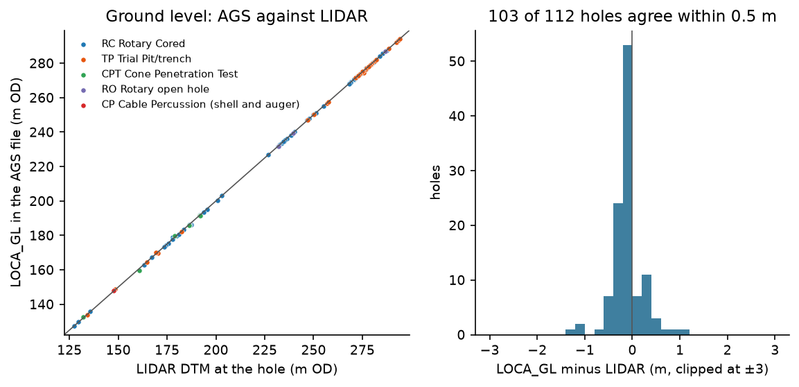
The agreement is good. The surveyed levels sit a median 0.13 m below the LIDAR, about what you would expect from 2 m cells that average the ground around each hole. Only three holes are more than 1 m out, and the DTM shows why. TP602, CP204 and CP106 stand on slopes of 8°, 9° and 18°, where the median slope at the holes is 4°, and the ground within 5 m of each varies by 1.6 to 2.1 m. On ground that steep, a few metres of difference between the surveyed position and the 2 m cell makes a metre of difference in level. None of the three is far enough out to suggest a hole in the wrong place.
Step 5: draw the maps
Both maps use the LIDAR as their basemap: a hillshade from matplotlib’s LightSource, with the DTM tinted on top. Every map carries the data credit in its corner. The first map, at the top of this post, colours holes by type. The second colours each hole by the first bedrock formation it meets:
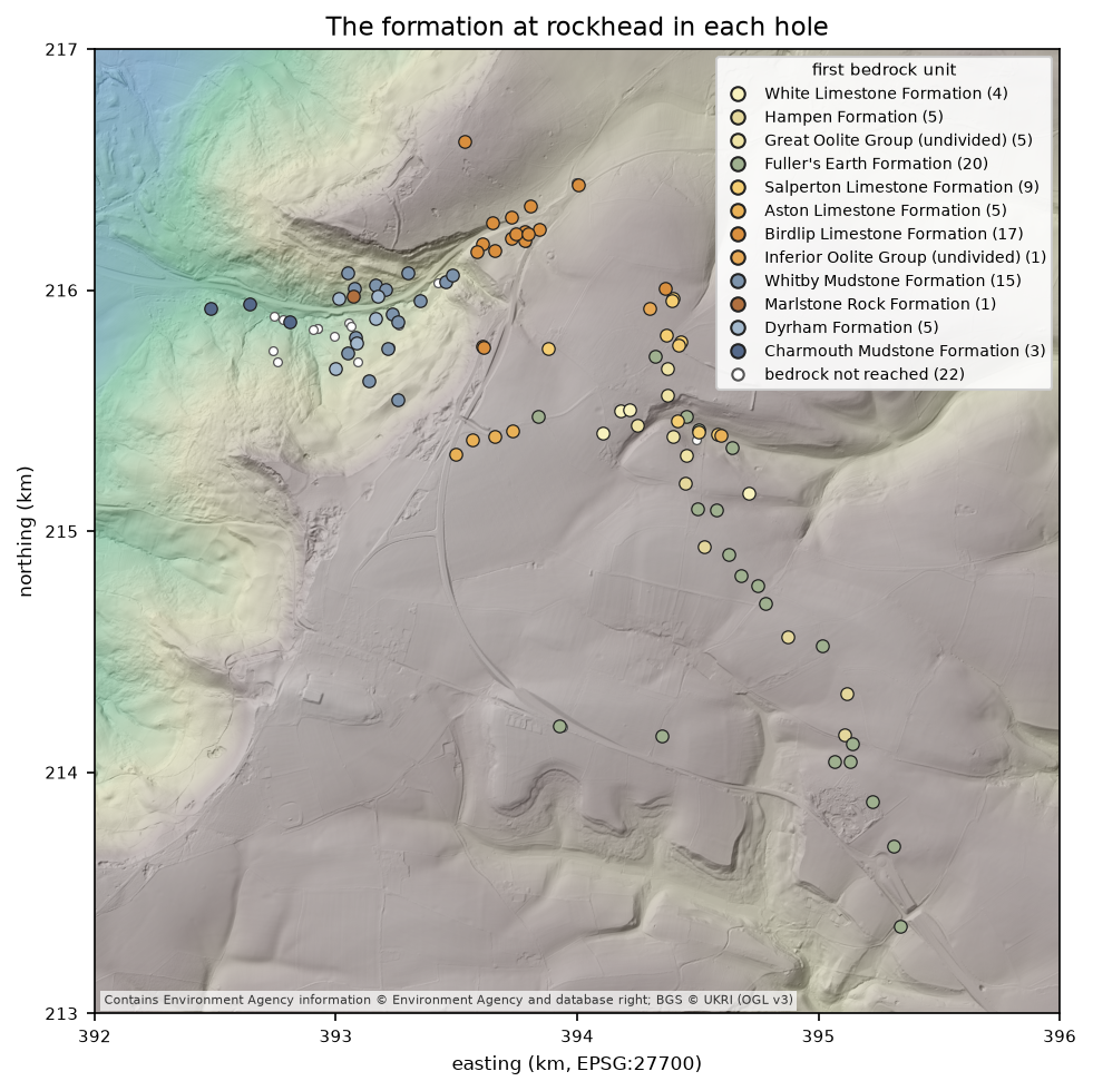
Even as points this is a geological map. Going up the hill from the vale, the holes meet the Charmouth Mudstone and Dyrham Formation, then the Whitby Mudstone, then the Inferior Oolite limestones of the scarp face, and finally the Fuller’s Earth and Great Oolite of the plateau, each younger than the last. That is the gently dipping Jurassic of the Cotswold escarpment, recovered from nothing but GEOL.
Step 6: a GeoPackage and a QGIS project
The script writes the points with 19 attribute fields to a GeoPackage, plus the DTM and hillshade as GeoTIFFs:
=== Step 6: write a GeoPackage for QGIS ===wrote output/a417_boreholes.gpkg: layer 'boreholes', 112 points, 19 fields, CRS 27700rasters for the QGIS basemap: a417_dtm_2m.tif, a417_hillshade.tifYou could style those by hand in QGIS, but qgis_borehole_map.py does it with PyQGIS, so the project can be rebuilt whenever the data changes. Run it with the Python that comes with QGIS. On Windows that is python-qgis-ltr.bat in the QGIS bin folder:
"C:\Program Files\QGIS 3.40.12\bin\python-qgis-ltr.bat" qgis_borehole_map.pyIt gives each hole type its own symbol, labels every hole with its LOCA_ID on a white halo, and sets a map tip: an HTML template that QGIS fills in from the feature under the mouse. Expressions in [% %] are evaluated, so the template can format numbers and leave out lines that don’t apply:
MAP_TIP = """<div style="font-family:sans-serif;font-size:12px;min-width:260px"><b style="font-size:14px">[% "LOCA_ID" %]</b> · [% "type_name" %]<br>Ground level [% format_number("LOCA_GL", 2) %] m OD (LIDAR [% format_number("lidar_gl", 2) %])<br>Final depth [% format_number("LOCA_FDEP", 2) %] m[% CASE WHEN "rockhead_depth" IS NOT NULL THEN '· rock at ' || format_number("rockhead_depth", 2) || ' m (' || "rockhead_name" || ')' END %]<br>[% CASE WHEN "first_water_strike" IS NOT NULL THEN 'First water strike ' || format_number("first_water_strike", 2) || ' m<br>' END %][% "n_samples" %] samples, [% "n_spt" %] SPTs<hr style="margin:4px 0">[% "log_html" %]</div>"""The script also records the data credits, as layer attribution and as the project’s copyright label (View > Decorations > Copyright Label), so every map exported from the project carries them. It saves output/a417_boreholes.qgz and renders the top of Crickley Hill, where the holes are densest:
QGIS 3.40.12-Bratislavahillshade valid=True | boreholes valid=True, 112 features, CRS EPSG:27700saved output/a417_boreholes.qgz with the style, labels and map tiprendered 04-qgis-borehole-map.png at 1:4,724; render errors: 0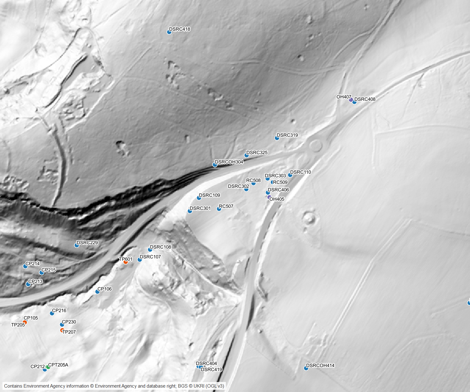
Open the project in QGIS Desktop, turn on View > Show Map Tips, and hover over a hole:
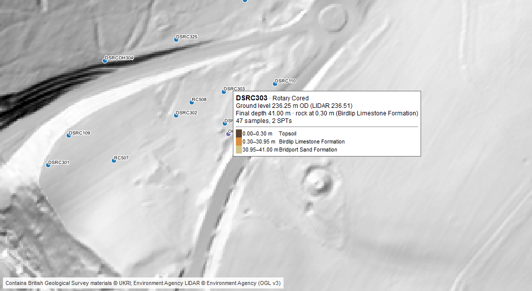
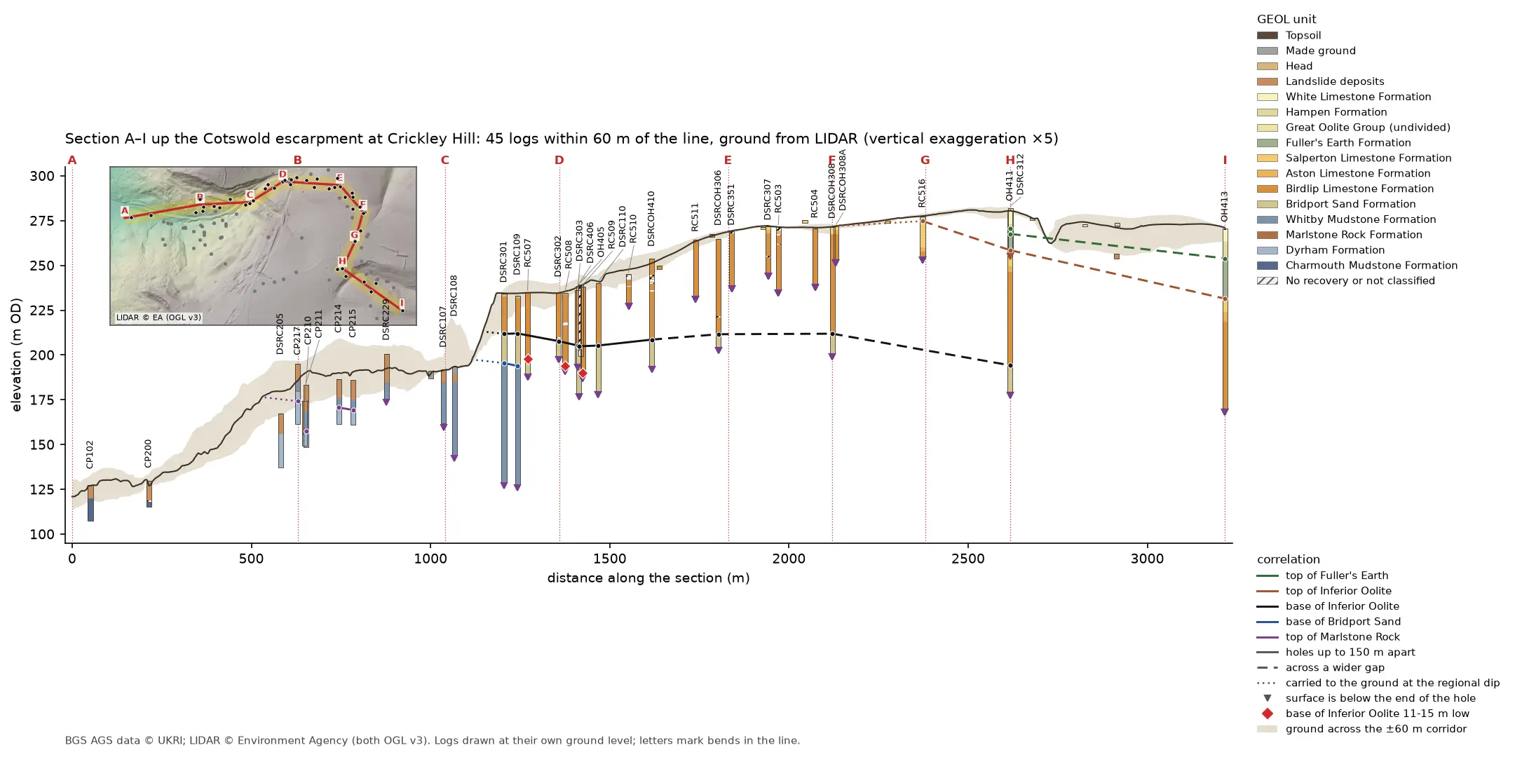
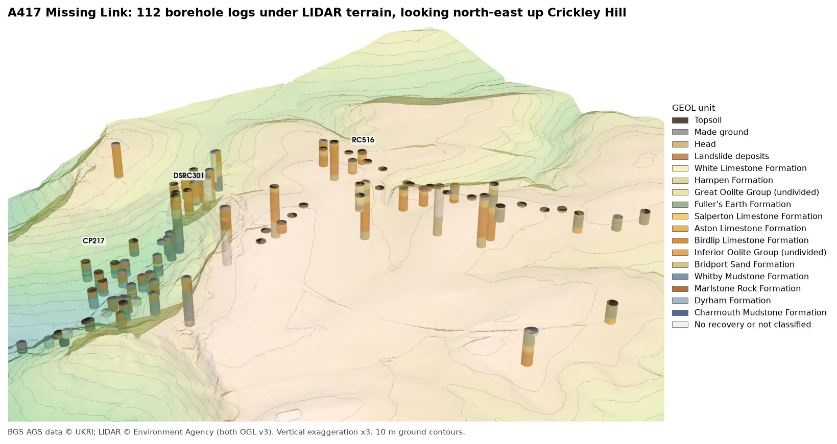
DSRC303 goes straight from 0.30 m of topsoil into 30.65 m of Birdlip Limestone and then the Bridport Sand. Hovering along the line of holes shows the base of the limestone changing from hole to hole, and Part 3 looks at that in 3D.
Frequently asked questions
What CRS do AGS coordinates use?
In UK files, LOCA_NATE and LOCA_NATN are British National Grid eastings and northings in metres (EPSG:27700). Check LOCA_GREF to be sure: some files use the Irish Grid, a local site grid in LOCA_LOCX and LOCA_LOCY, or latitude and longitude in LOCA_LAT and LOCA_LON.
Why are my boreholes in the sea?
Usually the easting and northing have been swapped. If they don’t appear at all, they have probably been treated as longitude and latitude, which gives “longitudes” in the hundreds of thousands. Make the points from LOCA_NATE as x and LOCA_NATN as y, and set EPSG:27700.
How do I get LIDAR ground levels for a site in England?
The Environment Agency publishes its LIDAR composite DTM through the Defra Data Services Platform as downloads and as a Web Coverage Service. The script requests 1 km tiles from the WCS and caches them, so it only downloads once.
How do I show a borehole log in a QGIS popup?
Build the log as an HTML table in one attribute field, then put that field into the layer’s map tip template (Layer Properties > Display). Turn on View > Show Map Tips and hover over a point.
Can I use a background map from the web instead?
Yes, as long as its licence allows you to publish maps made with it, and you show its attribution. OpenStreetMap (© OpenStreetMap contributors, ODbL) and Ordnance Survey OpenData (Open Government Licence) both do. Here the LIDAR hillshade shows the landforms that matter for the geology better than a street map would.
Next steps
- Part 3: 3D borehole logs builds every log as coloured cylinders in PyVista and in a QGIS 3D view, and tests whether neighbouring logs agree.
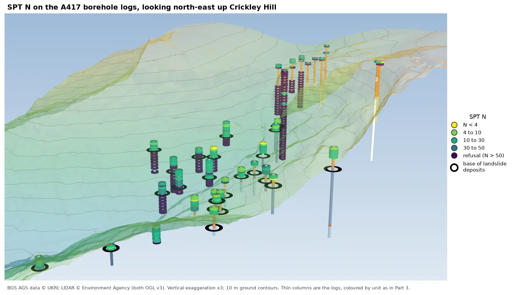
- Later in the series: cross-sections along a line of boreholes using this LIDAR for ground level, interpolated stratum surfaces such as rockhead, test results such as SPT N-values, and a 3D-printed ground model.
- For more on LIDAR itself, see LIDAR point clouds with laspy.
Data and licences
- A417 Missing Link ground investigation (BGS deposited data item 173984; client Highways England, now National Highways; contractor Geotechnical Engineering Ltd), downloaded through the BGS AGS borehole index and export APIs. Contains British Geological Survey materials © UKRI 2026, licensed under the Open Government Licence v3.0.
- Environment Agency LIDAR Composite DTM 1 m, requested at 2 m from the Defra Data Services Platform WCS. © Environment Agency copyright and/or database right, licensed under the Open Government Licence v3.0. The hillshade under every map in this post is made from it, and each map carries the credit. No third-party web map tiles are used.
- Code:
boreholes_map.py,qgis_borehole_map.pyanda417_ags.py, tested with Python 3.12.0, python-ags4 1.2.0, GeoPandas 1.2.0, rasterio 1.5.2, pyproj 3.8.0, matplotlib 3.11.2 and QGIS 3.40.12.
Key terms
- British National Grid
- The Ordnance Survey's grid for Great Britain (EPSG:27700), with eastings and northings in metres. AGS LOCA_NATE and LOCA_NATN use it in UK investigations.
- LOCA_GL
- The ground level at an exploratory hole, in metres above Ordnance Datum, as recorded in the AGS LOCA group.
- LIDAR DTM
- A digital terrain model from airborne laser scanning, showing the bare ground with buildings and vegetation removed.
- Map tip
- QGIS's hover popup. Its HTML template can include field values and expressions, so it can show a formatted borehole summary.
Data for this tutorial
- BGS AGS borehole data · Donated AGS ground investigation data, Open Government Licence
Licences and formats for each source are listed in the GIS data sources catalogue.